|
The Open FUSION Toolkit 26.6
An open-source framework for fusion and plasma science and engineering
|
Loading...
Searching...
No Matches
|
The Open FUSION Toolkit 26.6
An open-source framework for fusion and plasma science and engineering
|
ThinCurr solves variants of a system of equations corresponding to inductive-resistive dynamics of currents flowing in thin conducting structures (2D sheets in 3D geometry)
\[ \mathrm{L} \frac{\partial I}{\partial t} + \mathrm{R} I = V. \]
ThinCurr should primarily be used through the python interface using the OpenFUSIONToolkit.ThinCurr python module and the OpenFUSIONToolkit.ThinCurr.ThinCurr class.
The following examples illustrate usage of ThinCurr to perform calculations using the thin-wall model.
Python interface (recommended)
Command line interface (deprecated)
Driver-specific settings groups are defined for each of the programs above (eg. thincurr_td), follow links for description of available settings.
The following driver-wide settings are also available:
Option group: thincurr_hodlr_options (see HODLR)
| Option | Description | Type [dim] |
|---|---|---|
| target_size=1500 | Target size for mesh partitioning | int |
| aca_min_its=20 | Minimum nuber of ACA+ iterations to perfom (if used) | int |
| L_svd_tol=-1.0 | SVD tolerance for HODLR compression of \( \textrm{L} \) matrix (negative to disable) | int |
| L_aca_rel_tol=-1.0 | ACA tolerance (relative to SVD) for HODLR compression of \( \textrm{L} \) matrix (negative to disable) | int |
| B_svd_tol=T | SVD tolerance for HODLR compression of B reconstruction operator (negative to disable) | int |
| B_aca_rel_tol=F | ACA tolerance (relative to SVD) for HODLR compression of B reconstruction operator (negative to disable) | int |
Settings for ThinCurr runs are contained in the oft->thincurr element, with the following elements:
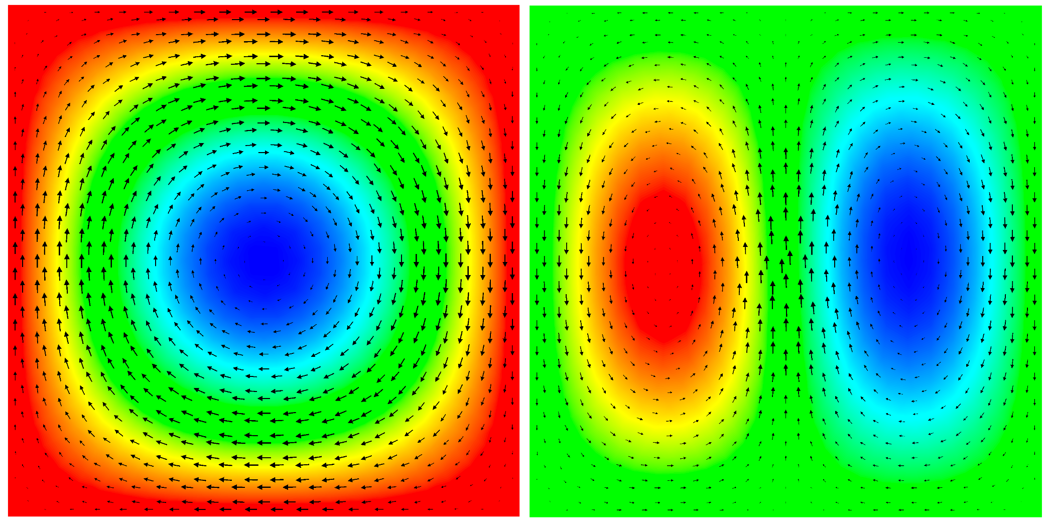
Currents in ThinCurr are represented in terms of a surface current ( \( \textbf{J}_s = \int \textbf{J} dt_w = \textbf{J} * t_w \)), where \( t_w \) is the direction through the thickness of the wall, represents a uniform current flowing in a wall of approximately zero thickness. To produce a convienient basis that satisfies \( \nabla \cdot \textbf{J}_s = 0 \), a surface potential is used such that \( \textbf{J}_s = \nabla \phi \times \hat{\textbf{n}} \), where \( \hat{\textbf{n}} \) is the unit normal on the surface. \( \phi \) is then expanded in a scalar Lagrange basis
\[ \textbf{J}_s (\textbf{r}) = \sum_j \alpha_j \phi_j (\textbf{r}) \times \hat{\textbf{n}} \]
on an unstructured triangular grid. Additional filament elements can also be defined to represent coils and other suitable structures. With these preliminaries a Boundary Finite Element Method (BFEM) is then used to define the inductance \( \mathrm{L} \) and resistance \( \mathrm{R} \) operators as
\[ \mathrm{L}_{i,j} = \frac{\mu_0}{4 \pi} \int_{\Omega} \int_{\Omega'} \left( \nabla \phi_i (r) \times \hat{\textbf{n}} \right) \cdot \frac{\nabla \phi_j (r') \times \hat{\textbf{n}}}{|\textbf{r}-\textbf{r}'|} dA' dA \]
and
\[ \mathrm{R}_{i,j} = \int_{\Omega} \eta_s(r) \left( \nabla \phi_i (r) \times \hat{\textbf{n}} \right) \cdot \left( \nabla \phi_j (r) \times \hat{\textbf{n}} \right) dA, \]
yielding the final discretized system
\[ \mathrm{L}_{i,j} \frac{\partial \alpha_j}{\partial t} + \mathrm{R}_{i,j} \alpha_j = V_i, \]
where \( \alpha_j \) and \( V_i \) are the finite element weights and externally-applied voltages respectively. Voltages can be directly applied to filament elements or through the action of defined current waveforms through inductive coupling as in \( \mathrm{L} \).
In addition to the meshed surfaces, conducting structures can also be represented using filaments. Filaments can have fixed current (icoils) or voltage (vcoils) waveforms as a function of time. In the latter case, resistance per unit length and effective radius can be specified for calculating self-inductance and resistive dissipation. For coupling between filaments and other filaments and surface elements zero cross-sectional area is assumed (ie. a simple line integral).
Note that for icoils the current in a given coil_set is fixed, but the voltage on the coil will vary according to the mutual coupling of all coils and surfaces. Conversely, for vcoils the voltage is fixed and the current evolution will vary consistent with the mutual coupling of all coils and surfaces and the coils self-inductance and resistivity.
The icoils element should contain one or more coil_set elements each with one or more coil elements.
If two values are given for inside a coil element, they are treated as the R,Z position of a circular coil. If a general 3D coil is desired, the number of points may be specified using the npts attribute and a corresponding list of points (1 per line) provided in the element with comma-separated X,Y,Z positions.
The vcoils element should contain one or more coil_set elements each with one or more coil elements.
As above, if two values are given for inside a coil element, they are treated as the R,Z position of a circular coil. If a general 3D coil is desired, the number of points may be specified using the npts attribute and a corresponding list of points (1 per line) provided in the element with comma-separated X,Y,Z positions.
At the edge of a surface a boundary condition is required to ensure that no current flows normal to the boundary, which would result in divergence or lost current. By considering the potential representation we can easily show that zero normal current is satisfied by the condition \( | \nabla \phi \times \hat{\textbf{n}} \times \hat{\textbf{t}} | = | \nabla \phi \cdot \hat{\textbf{t}} | = 0\), where \( \hat{\textbf{t}} \) is the unit normal in the direction tangential to the boundary. This amounts to the condition that \( \phi \) is a constant on a given boundary. A simple solution that satisfies this boundary condition is to set the value on all boundary nodes to a single fixed value (generally zero). However as we will see in the next section this is overly restrictive for many cases.

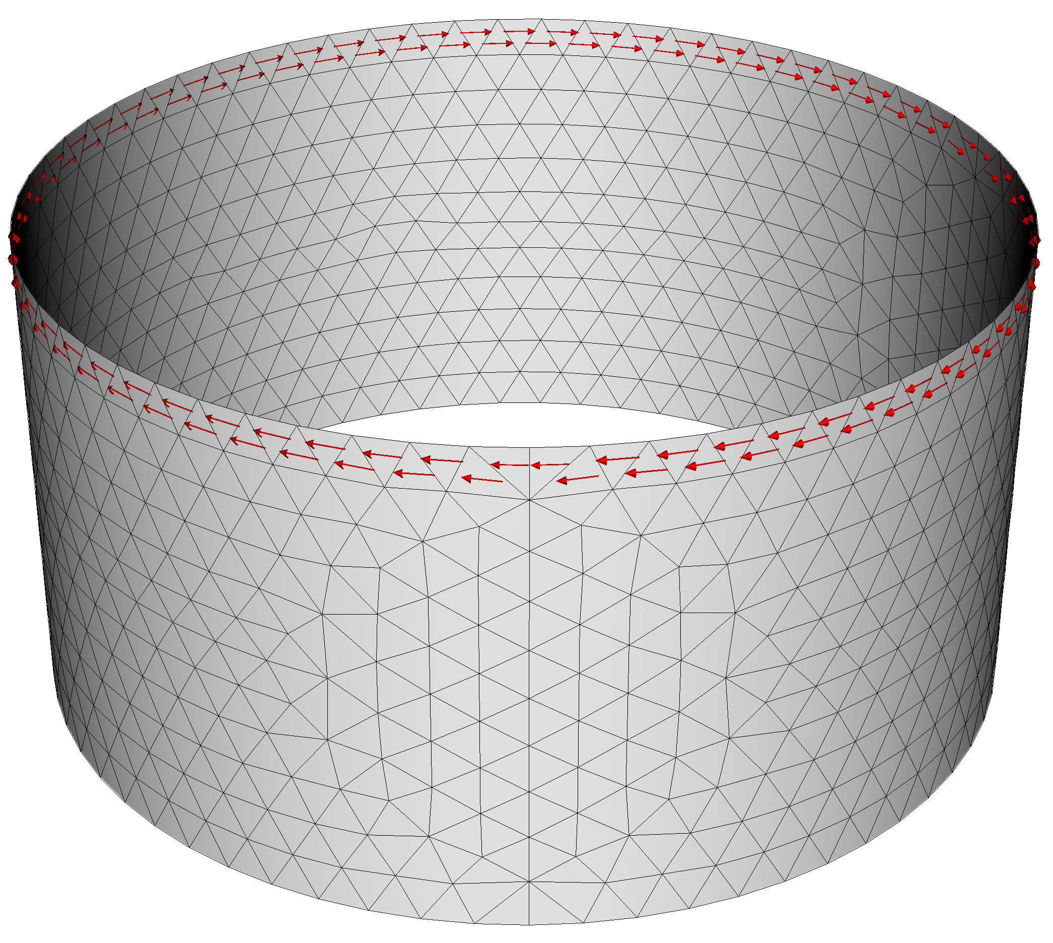
Note the boundary condition above requires a constant potential on a given boundary. However, for multiply connected geometry, such as a cylinder, one or more distinct boundaries exist such that the potential can be different on each boundary. For the case of the cylinder there are two geometrically distinct boundarys, the top and bottom circular edges. If we consider the potential formulation we can show that the current flow across a line between two points on a given surface is given by the difference in the potential between those points
\[ \mathrm{I}_{l} = \int_a^b \hat{\textbf{n}} \cdot (\nabla \phi \times \hat{\textbf{n}} \times \textbf{dl}) = \int_a^b \nabla \phi \cdot \textbf{dl} = (\phi_b - \phi_a). \]
So if point \( a \) and \( b \) exist on different boundaries then the difference in the constant for each boundary defines the current passing between them. In the case of the cylinder this corresponds to the total current flowing azimuthally around the cylinder.
To enable the values on boundaries to vary self-consistently in the model we define a new element that corresponds to a constant potential on a given closed boundary loop. In ThinCurr we call these elements "holes", as they are related to the topological concept of "holes". These elements correspond to current flowing around the boundary loop, and correspondingly to capturing magnetic flux within this loop. This captures flux that links the mesh without crossing through any of the triangles themselves (eg. flux down the center of a cylinder).
While one may think we should add two holes in the case of the cylinder this is not the case as it would introduce a gauge ambiguity in the system, resulting in a singular \( \textbf{L} \) matrix. We can see this by considering the azimuthal flowing current, which as above is given by the difference in potential between the top \( \phi_a \) and bottom \( \phi_b \) of the cylinder. This means that a single current in our model is dependent on two values, indicating a redundancy that means \( \textbf{L} \) is not full rank, or in other words singular. To avoid this we only introduce only one hole, which in turn sets the potential on the other boundary to zero and eliminates the gauge ambiguity.
Multiply connected regions:
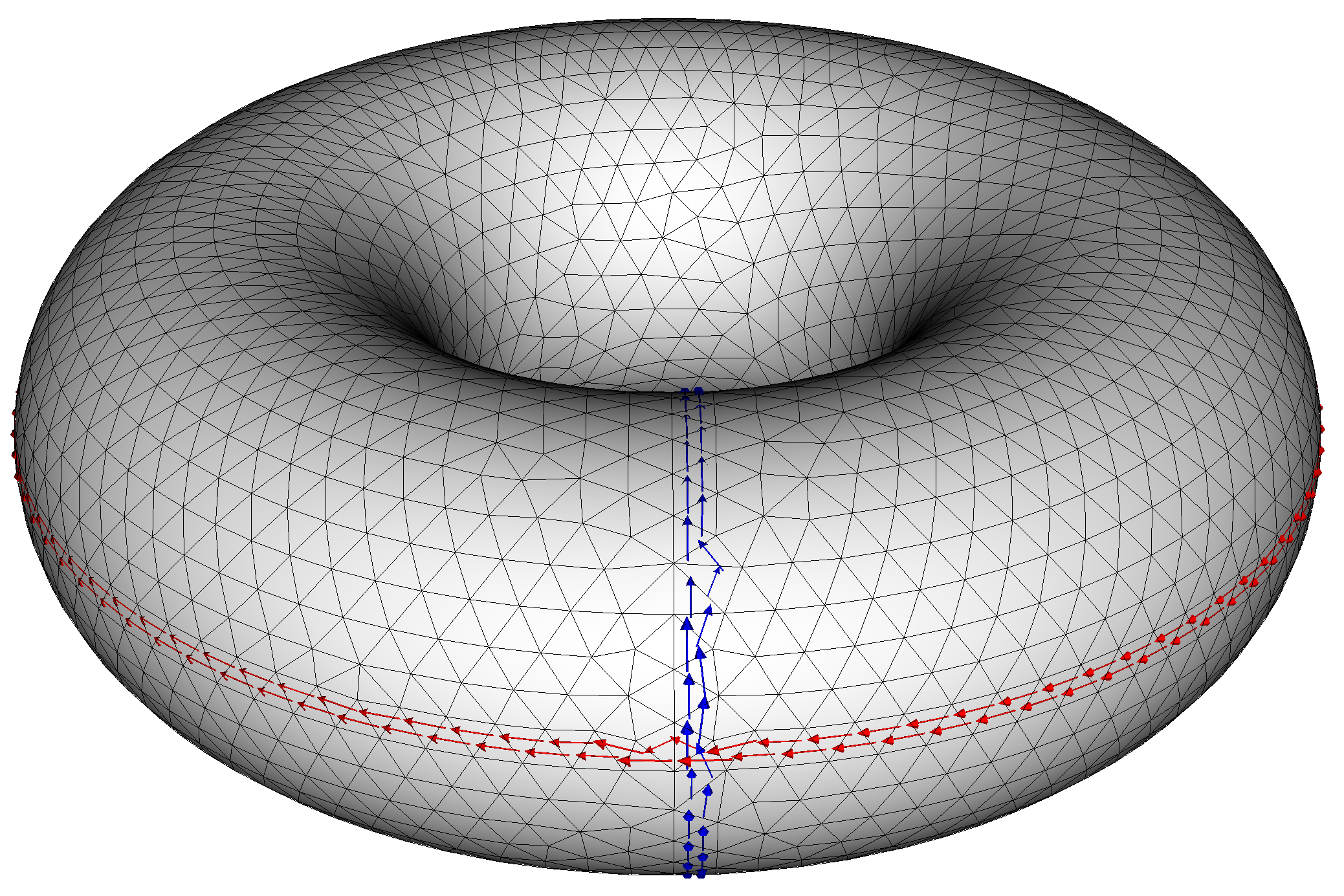
Hole elements are not just necessary when there is a visible boundary, but whenever there are multiple distinct topological paths on a given surface. An example of this case is the torus, where there are two topologically distinct paths corresponding to the short (poloidal) and long (toroidal) way around the torus. We can see this using the consideration of the difference in potentials above, as the potential difference between any two points will always be zero and as a result no net current can flow in the poloidal or toroidal directions. To correct this two holes must be added, corresponding to loops in each of these two directions, which makes \( \phi \) mutlivalued so that a difference in potential can exist even on closed paths. This use of jumps and a single-valued potential to represent a multivalued potential is common practice in numerical methods.
Holes can be defined using the ThinCurr_compute_holes.py script. This script analyzes the toplogy of a given mesh and automatically locates and defines needed hole elements. This is now the recommended way of defining holes in ThinCurr models, although manual definition is also still supported.
As stated above the fact that the solution depends only on the gradient and not on the absolute value of \( \phi \) itself can introduce a gauge ambiguity, resulting in redundant degrees of freedom. In the cases considered above this is resolved by keeping the potential on at least one boundary fixed to zero. However, when a surface is fully closed, as is the case for a sphere or torus, there are no boundaries. So to fix the gauge on these surfaces we must remove an element from the system, effectively fixing the potential to zero at that point. We call these elements "closure" elements as they are used to close the system, making it solveable.
As with holes, closures can also be defined using the ThinCurr_compute_holes.py script. This is now the recommended way of defining closures in ThinCurr models, although manual definition is also still supported.
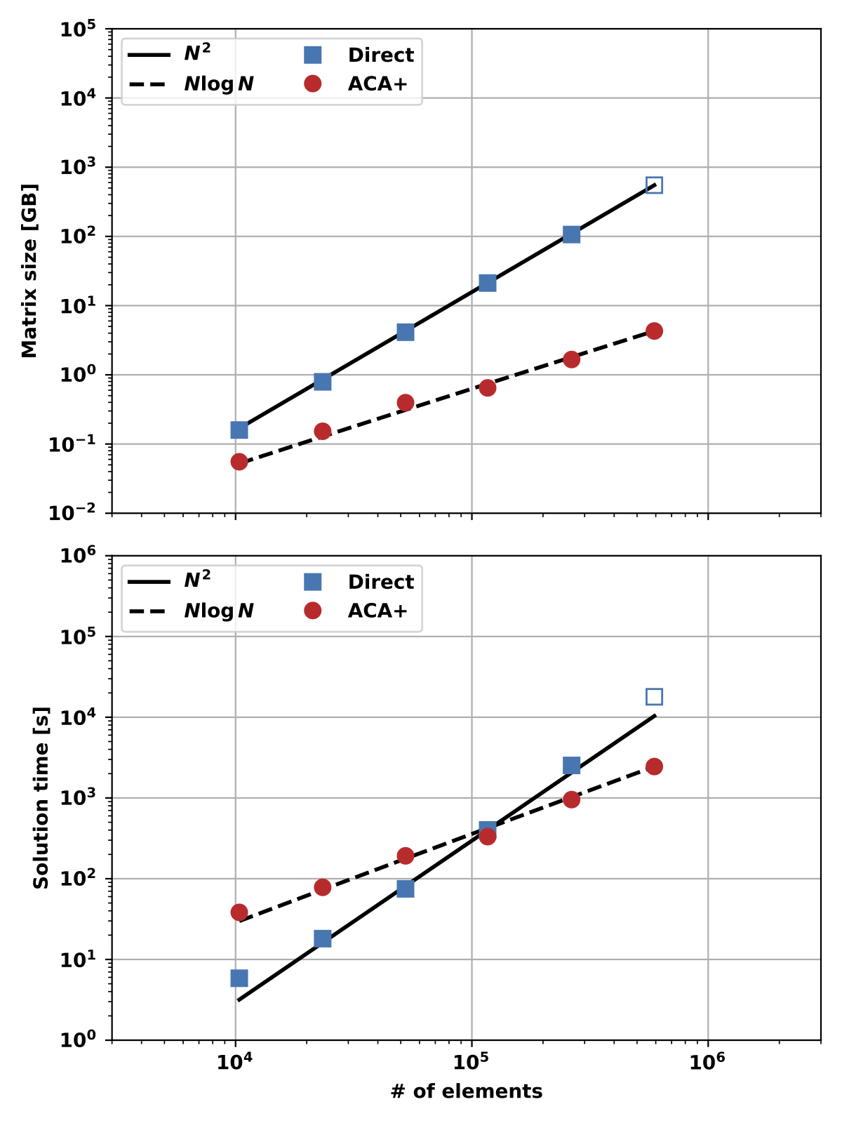
In the standard BFEM approach described above every element interacts with every other element, leading to a dense \( \textrm{L} \) and growth of memory and time requirements at a rate of \( O(N^2) \), where \( N \) is the number of elements in the model. This limits the size of models on most systems to < 20k elements on a typical laptop with 16GB of RAM and < 180k on even a large workstation with 1TB of RAM. In addition to memory limits, these models will take a very long time to compute as the number of FLOPs required will also scale as \( O(N^2) \).
To avoid this ThinCurr models can take advantage of the structure of the \( \textrm{L} \) matrix to generate an approximation of the full matrix with some desired tolerance. As application of these models to engineering and other studies often do not require extremely high accuracy, this can dramatically reduce the computational requirement while retaining sufficient fidelity for a desired study. This is possible as the \( \textrm{L} \) constructed from the BFEM exhibits a low-rank structure for interactions between elements that are physically separated by a large distance relative to their size. If we spatial partition our mesh into regions, the interactions between separate regions, so called off-diagonal blocks of the matrix, will possess this low-rank structure, meaning they can be well approximated by a matrix with smaller rank (eg. truncated SVD). To improve efficiency and performance such a spatial partitioning can be done in a nested fashion, leading to a so-called Hierarchical Off-Diagonal Low-Rank (HODLR) approximation to the matrix.
ThinCurr currently utilizes a binary tree to partition the surface mesh used to discretize currents in the model. Initially, a bounding box is created that encloses the full mesh. The mesh is then recursively subdivided by looking at each partition and subdividing it in one of the three principal cartesian directions if the number of elements is greater than a given size (target_size). On each level, the direction of subdivision is chosen to be the direction with largest standard deviation of position over the contained points. Near and far interactins between mesh regions are then determined on each level, taking into account appropriate "masking" of interactions from higher levels.

Once the spatial partitioning is complete the individual matrix blocks can be constructed. First, diagonal blocks are fully assembled and stored as dense matrices. Next, low-rank approximations are computed for all off-diagonal blocks. For blocks whose corresponding mesh regions are "close" to eachother, as determined by the ratio of the center-center separation to the circumradius of each region, the full block is computed and then compressed using an SVD. The compression is set by truncating the SVD at a user-specified tolerance (specified by L_svd_tol), based on the Frobenius norm of the singular values.
For all other blocks, which correspond to off-diagonal blocks whose corresponding mesh regions are not "close" to eachother the Adaptive Cross-Appoximation technique is used. This technique iteratively builds a low-rank approximation ( \( \textrm{M} \approx \textrm{U} \textrm{V}^T \)) by sampling rows and columns of the block and stopping once a desired tolerance, defined relative to the SVD tolerance (L_aca_rel_tol < 1.0), has been reached. As ACA+ has some inherent random variation, the tolerance specified for ACA+ should be higher than the SVD tolerance (L_aca_rel_tol < 1.0). After a block's approximation by ACA+ is complete the resulting block is then recompressed using SVD for greater run to run consistency.