|
The Open FUSION Toolkit 26.6
An open-source framework for fusion and plasma science and engineering
|
Loading...
Searching...
No Matches
|
The Open FUSION Toolkit 26.6
An open-source framework for fusion and plasma science and engineering
|
In this example we demonstrate how to compute eigenvalues and eigenvectors for a simple ThinCurr model.
To load the ThinCurr python module we need to tell python where to the module is located. This can be done either through the PYTHONPATH environment variable or within a script using sys.path.append() as below, where we look for the environement variable OFT_ROOTPATH to provide the path to where the OpenFUSIONToolkit is installed (/Applications/OFT for binaries on macOS).
We now create a OFT_env instance for execution using two threads and a ThinCurr instance that utilizes that execution environment.
Once created, we setup the model from an existing HDF5 and XML mesh definition using setup_model().
Finally, we initialize I/O for this model using setup_io() to enable output of plotting files for 3D visualization in VisIt, Paraview, or using pyvista below.
#----------------------------------------------
             ____  ____________
            / __ \/ ____/_  __/
           / / / / /_    / /
          / /_/ / __/   / /
          \____/_/     /_/

Base release:        v1.0.0-beta7
Development branch:  release_26_06
Revision id:         978c4b9f

Parallelization Info:
  Not compiled with MPI
  # of OpenMP threads =    2

Linear Algebra backend: native

#----------------------------------------------


Creating thin-wall model
  No V(t) driver coils found
  Loading I(t) driver coils
    Masked      0 coils from sensors
  Building holes

  Loading region surface resistivity:
     1  1.2570E-05

  Setup complete:
    # of points    =          492
    # of edges     =         1393
    # of cells     =          902
    # of holes     =            0
    # of closures  =            0
    # of Vcoils    =            0
    # of Icoils    =            1
With the model setup, we can now compute the self-inductance and resistivity matrices. A numpy version of the self-inductance matrix will be stored at tw_plate.Lmat. By default the resistivity matrix is not moved to python as it is sparse and converting to dense representation would require an increase in memory. These matrices correspond to the \(\textrm{L}\) and \(\textrm{R}\) matrices for the physical system
\(\textrm{L} \frac{\partial I}{\partial t} + \textrm{R} I = V\)
Building element<->element self inductance matrix
  Time =  0s
Building resistivity matrix
With \(\textrm{L}\) and \(\textrm{R}\) matrices we can now compute the eigenvalues and eigenvectors of the system \(\textrm{L} I = \lambda \textrm{R} I\), where the eigenvalues \(\lambda = \tau_{L/R}\) are the decay time-constants of the current distribution corresponding to each eigenvector.
Starting eigenvalue solve (ARPACK)
  Time =   3.2170E-03
  Eigenvalues
      9.732856E-03
      6.530427E-03
      6.530315E-03
      5.250082E-03
      4.703101E-03
The resulting currents can be saved for plotting using tw_plate.save_current(). Here we save each of the five eigenvectors for visualization. Once all fields have been saved for plotting tw_plate.build_XDMF() to generate the XDMF descriptor files for plotting with VisIt of Paraview. This method also returns a XDMF_plot_file object, which can be used to read and interact with plot data in Python (see below).
Creating output files: oft_xdmf.XXXX.h5
  Removing old Xdmf files
    Removed 2 files
  Found Group: thincurr
    Found Mesh: icoils
    Found Mesh: smesh
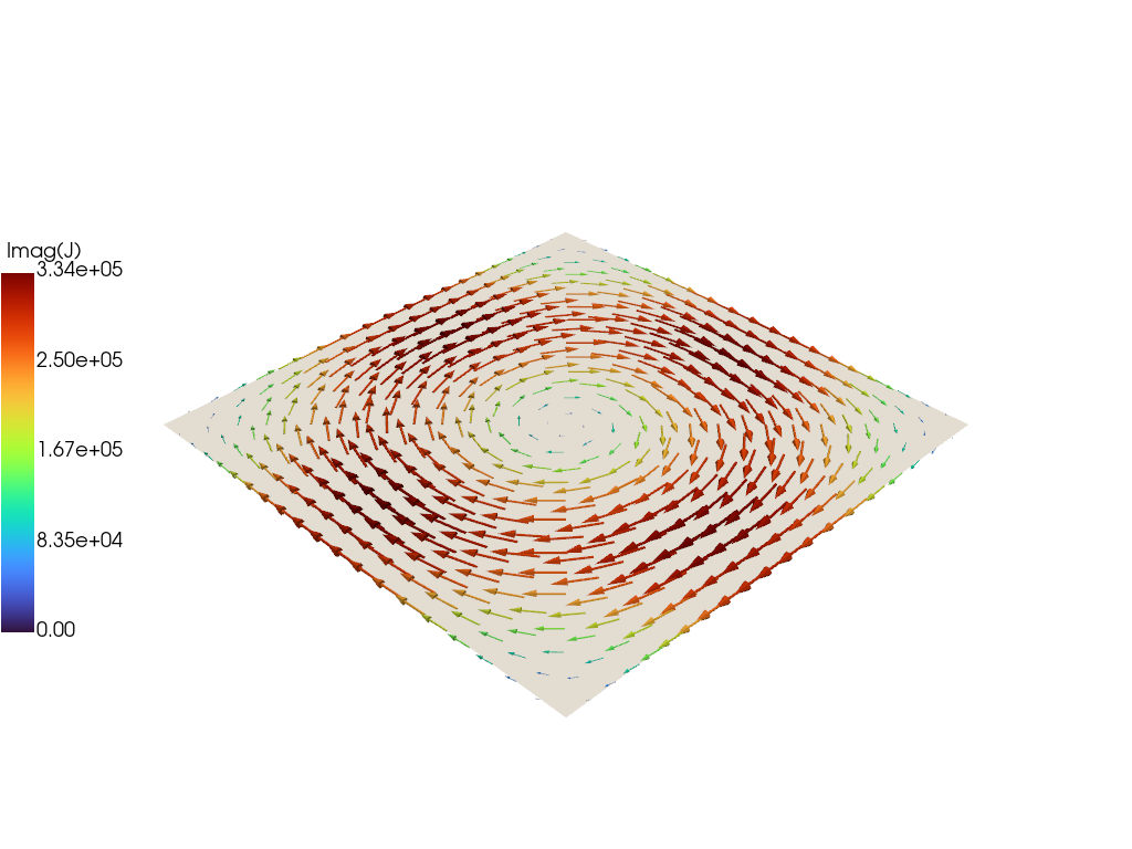
Finally we plot the current vectors on the plate showing the longest-lived eddy current structure, which corresponds to a large circulation on the plate. The XDMF_plot_file class provides functionality to work with the data stored in OFT plot files, including methods to generate information for 3D plotting in Python using pyvista.
Plotting data is always associated with a specific mesh, which is itself associated with a physics group. In this case ThinCurr is the physics group and the data we are interested in is stored on the surface mesh smesh. The plot_data['ThinCurr']['smesh'] is a XDMF_plot_mesh object with further functionality for accessing data.
To plot the first eigenvector we first get the pyvista plotting grid using get_pyvista_grid() and then retrieve the vertex-centered field (J_01_v) using get_field()