Running a frequency-response calculation

To run a frequency-response calculation we use similar workflow to ThinCurr Example: Eigenstates of a square plate and ThinCurr Example: Time-dependent model of a cylinder. In this case the frequency-response calculation uses two icoil sets, where the sets correspond to the real and imaginary components of the source respectively. For this case we have a single icoil set, composed of two circular coils (R,Z location defines the coil) with opposite polarities set by the scale attribute.

With the two input files defined we can use thincurr_fr to run a frequency-response calculation.

/path/to/OFT/bin/thincurr_fr oft.in oft_in.xml

Contents of the input files are provided below and in the examples directory under ThinCurr/torus, along with the necessary mesh file thincurr_ex-torus.h5.

Post processing

Once complete you can now generate XDMF files suitable for visualization of results using the VisIt code. For frequency-response calculations we do not need to do a separate plotting run, so once complete, you just need to run the build_xdmf.py script, which generates XDMF metadata files that tells VisIt how to read the data. This can be done using the following command

python /path/to/oft/bin/build_xdmf.py

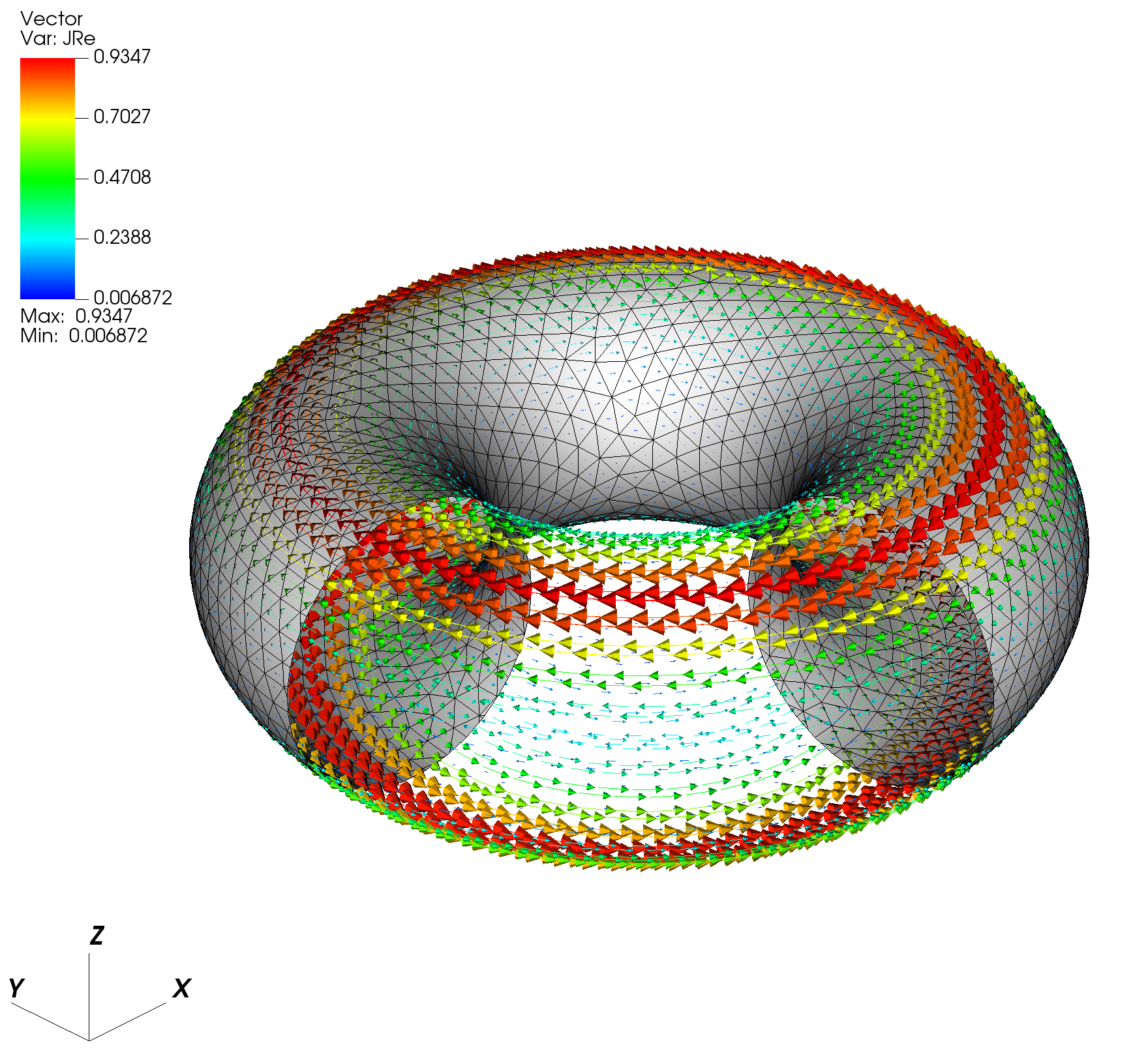
Next use VisIt to open the surf_static.xmf file, which will contain two vector fields JRe and JIm that correspond to the current distributions for the real and imaginary components of the solution in the frequency-domain. If you are running this example remotely and using VisIt locally you will need to copy the mesh.*.h5, scalar_dump.*.h5, vector_dump.*.h5, and *.xmf files to your local computer for visualization. The real component JRe should look like the figure below.

Resulting current distribution for the real part of the frequency response at f = 5 kHz

Supporting information

Input files

General global settings (oft.in)

&runtime_options
 debug=0
/

&mesh_options
 cad_type=0
/

&native_mesh_options
 filename="thincurr_ex-torus.h5"
/

&thincurr_fr_options
 direct=T
 freq=5.E3
 fr_limit=0
/

XML global settings (oft_in.xml)

<oft>
  <thincurr>
    <eta>1.257E-5</eta>
    <icoils>
      <coil_set>
        <coil scale="1.0">1.1, 0.25</coil>
        <coil scale="-1.0">1.1, -0.25</coil>
      </coil_set>
    </icoils>
  </thincurr>
</oft>

Mesh definition

Note: For a torus we must define a two holes and a single singularity, see "Hole" elements and "Closure" elements for more information.

Cubit mesh script (thincurr_ex-torus.jou)

reset
undo off
 
#{mesh_size=0.1}
 
# Create simple 1x0.5 torus
create curve arc radius 0.5 center location 1 0 0  normal 0 1 0  start angle 0 stop angle 360
sweep curve 1  zaxis angle 360
 
# Generate mesh
set trimesher geometry sizing off
surface all scheme trimesh
surface all size {mesh_size}
mesh surface all
 
# Create mesh blocks
set duplicate block elements off
block 1 add surface 1
nodeset 1 add curve 2
nodeset 2 add curve 3
sideset 1 add tri 1
 
# Export grid
set large exodus file on
export Genesis  "thincurr_ex-torus.g" overwrite block 1

The file can then be converted to OFT's native mesh format using the convert_cubit.py script as

python /path/to/OFT/bin/convert_cubit.py --in_file=thincurr_ex-torus.g

which will yield the converted file thincurr_ex-torus.h5.

Table of Contents

Running a frequency-response calculation

Post processing

Supporting information

Input files

Mesh definition