|
The Open FUSION Toolkit 26.6
An open-source framework for fusion and plasma science and engineering
|
Loading...
Searching...
No Matches
|
The Open FUSION Toolkit 26.6
An open-source framework for fusion and plasma science and engineering
|
To run an eigenstate simulation (compute the characteristic L/R-decaying modes) you can issue the following command from within one of the run directories. Note, make sure plot_run=F in the thincurr_eig_options group.
/path/to/oft/bin/thincurr_eig oft.in oft_in.xml
Contents of the input files are provided below and in the examples directory under ThinCurr/plate, along with the necessary mesh file thincurr_ex-plate.h5.
During the run you will see it report a bunch of general information and then it will report the first few eigenvalues from the calculation. These values should all be purely real (no imaginary component) and should be decreasing in value from first to last. For this case the largest values should be around 9.7 ms.
In addition to the inputs used in ThinCurr Example: Eigenstates of a square plate we now also include the thincurr_hodlr_options block, which controls the operation of HODLR approximation. If this block is ommitted or L_svd_tol < 0 then the full matrix is constructed. If L_aca_tol < 0 then the full matrix is built, but SVD compression is used for off-diagonal blocks. This saves memory, but not computational time during the formation of the inductance matrix. If both L_svd_tol > 0 and 0 < L_aca_tol < 1 then ACA+ is used to compute non-adjacent off-diagonal terms, which are then recompressed using SVD. Adjacent off-diagonal terms are computed using SVD compression on the full matrix block.
The same is true for the B_* options, which correspond to the magnetic field reconstruction when both plot_run=T and compute_B=T.
General global settings (oft.in)
&runtime_options
 debug=0
/

&mesh_options
 cad_type=0
/

&native_mesh_options
 filename="thincurr_ex-ports.h5"
/

&thincurr_eig_options
 direct=F
 plot_run=F
 compute_B=T
 neigs=6
/

&thincurr_hodlr_options
 target_size=1200
 aca_min_its=20
 L_svd_tol=1.E-8
 L_aca_rel_tol=0.05
 B_svd_tol=1.E-3
 B_aca_rel_tol=0.05
/
XML global settings (oft_in.xml)
<oft>
  <thincurr>
    <eta>1.257E-5</eta>
    <coil_set>
      <coil>0.5, 0.1</coil>
    </coil_set>
  </thincurr>
</oft>
Once complete you can now generate XDMF files suitable for visualization of results using the VisIt code. This is a two step process. First, rerun the code as above but with plot_run=T in the thincurr_eig_options group. Once complete, you need to run the build_xdmf.py script, which generates XDMF metadata files that tells VisIt how to read the data. This can be done using the following command
python /path/to/oft/bin/build_xdmf.py
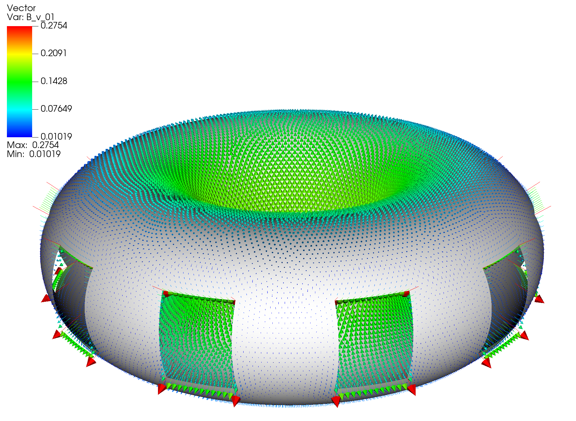
Next use VisIt to open the surf_static.xmf file, which will contain a series of vector fields named as J_XX and B_v_XX that correspond to the current distributions and magnetic field of the various eigenstates respectively. If you are running this example remotely and using VisIt locally you will need to copy the mesh.*.h5, scalar_dump.*.h5, vector_dump.*.h5, and *.xmf files to your local computer for visualization. The first eigenmode J_01 should look like the figure below.