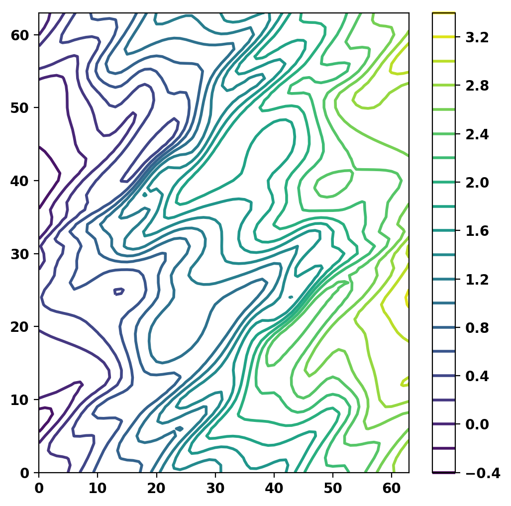
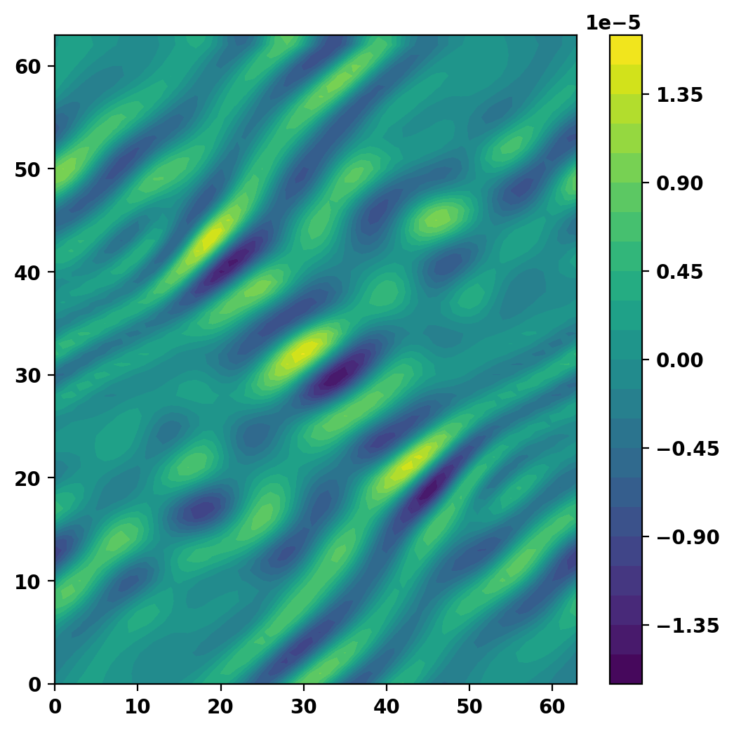
In this example we demonstrate how to compute a current potential on one surface that minimizes the error of the normal magnetic field on another. This is relevant to stellarator optimization when the normal field is minimized on a desired plasma surface and the current potential lies on a so-called winding surface here coils will be initialized for further optimization.

Note: Running this example requires the h5py python package, which is installable using pip or other standard methods.

import struct
import sys
import os
import numpy as np
import matplotlib.pyplot as plt
import matplotlib as mpl
plt.rcParams['figure.figsize']=(6,6)
plt.rcParams['font.weight']='bold'
plt.rcParams['axes.labelweight']='bold'
plt.rcParams['lines.linewidth']=2
plt.rcParams['lines.markeredgewidth']=2
%matplotlib inline
%config InlineBackend.figure_format = "retina"

Load ThinCurr library

To load the ThinCurr python module we need to tell python where to the module is located. This can be done either through the PYTHONPATH environment variable or within a script using sys.path.append() as below, where we look for the environement variable OFT_ROOTPATH to provide the path to where the OpenFUSIONToolkit is installed (/Applications/OFT for binaries on macOS).

thincurr_python_path = os.getenv('OFT_ROOTPATH')
if thincurr_python_path is not None:
    sys.path.append(os.path.join(thincurr_python_path,'python'))
from OpenFUSIONToolkit import OFT_env
from OpenFUSIONToolkit.ThinCurr import ThinCurr
from OpenFUSIONToolkit.ThinCurr.meshing import build_regcoil_grid, ThinCurr_periodic_toroid

Generate mesh and ThinCurr input for coil and plasma surfaces for NCSX

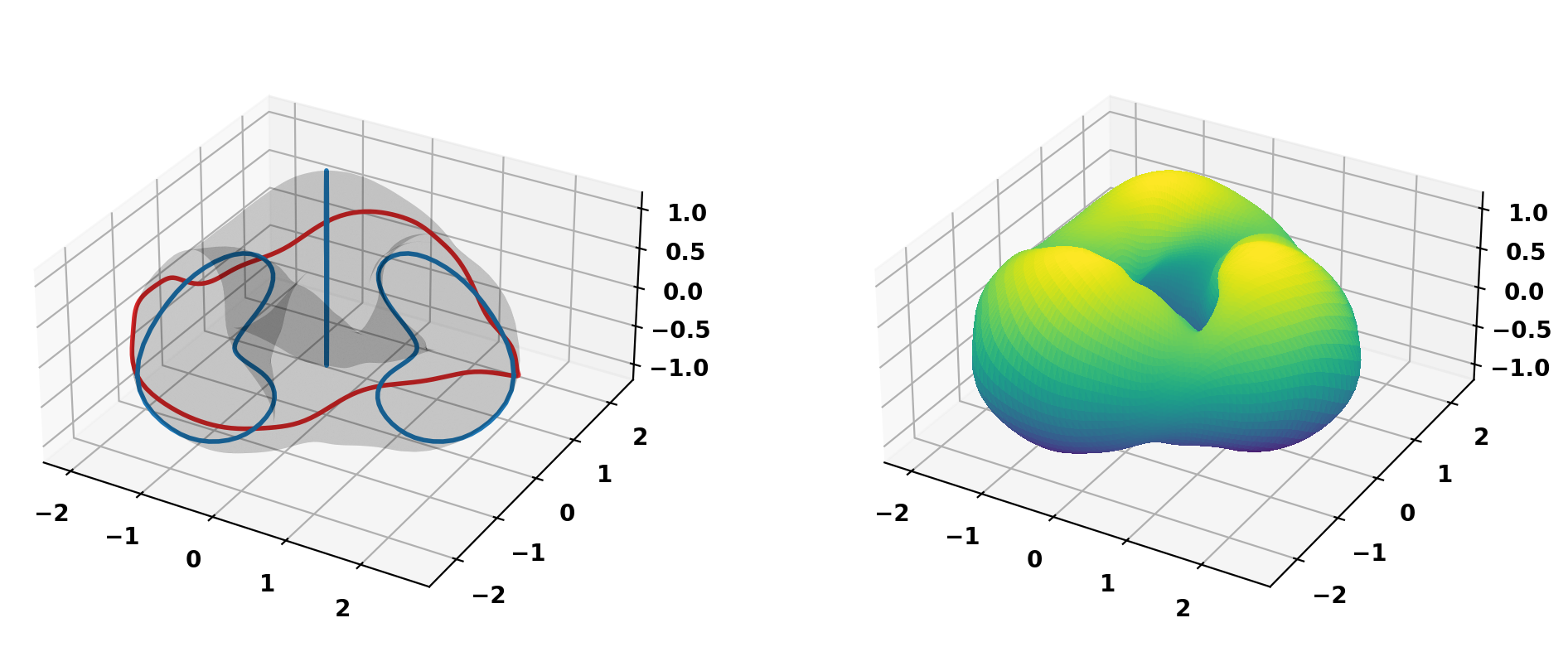
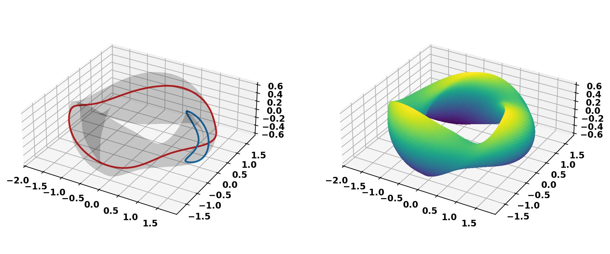
First we create ThinCurr models for the winding and plasma surfaces using a REGCOIL definition of the NCSX stellarator using build_regcoil_grid(). This subroutine builds a uniform grid over one field period, which can then be used by build_periodic_mesh() to build a mesh from the resulting grid. The result is a ThinCurr model, including periodicity mapping information (r_map).

We can now create ThinCurr models for the winding and plasma surfaces using a REGCOIL definition of the NCSX stellarator using build_regcoil_grid() and ThinCurr_periodic_toroid, which provides functionality for working with toroidally periodic meshes. The result are ThinCurr_periodic_toroid objects for the plasma (plasma_grid) and winding surface (coil_grid).

nphi = 64
ntheta = 64
# Create coil mesh
coil_grid, nfp = build_regcoil_grid('regcoil_out.li383.nc','coil',ntheta,nphi,full_torus=False)
coil_grid = ThinCurr_periodic_toroid(coil_grid,nfp,ntheta,nphi)
# Create plasma mesh
plasma_grid, _ = build_regcoil_grid('regcoil_out.li383.nc','plasma',ntheta,nphi,full_torus=True)
plasma_grid = ThinCurr_periodic_toroid(plasma_grid,1,ntheta,nphi)

Plot resulting winding surface mesh and save to file

fig = plt.figure(figsize=(12,5))
coil_grid.plot_mesh(fig)
coil_grid.write_to_file('thincurr_coil.h5')

Saving mesh: thincurr_coil.h5

Plot resulting plasma surface mesh and save to file

fig = plt.figure(figsize=(12,5))
plasma_grid.plot_mesh(fig)
plasma_grid.write_to_file('thincurr_plasma.h5')

Saving mesh: thincurr_plasma.h5

Compute optimal winding surface current

Setup ThinCurr model for winding surface

We now create a OFT_env instance for execution using four threads and a ThinCurr instance for the winding surface that utilizes that execution environment. Once created, we setup the model from an existing HDF5 and XML mesh definition using setup_model().

We also initialize I/O for this model using setup_io() to enable output of plotting files for 3D visualization in VisIt or Paraview.

In this case we specify a coil directory to use for saving I/O files to keep things separate for the other cases to be run in this notebook and in ThinCurr Python Example: Compute frequency-response in a torus.

Note: A warning will be generated that no XML node was found and a default resistivity value is being used. This is OK as we will not use the resitivity matrix with this model.

myOFT = OFT_env(nthreads=4)
tw_coil = ThinCurr(myOFT)
tw_coil.setup_model(mesh_file='thincurr_coil.h5')
tw_coil.setup_io(basepath='coil')

#----------------------------------------------
Open FUSION Toolkit Initialized
Development branch:   v1_beta6
Revision id:          681e857
Parallelization Info:
  # of MPI tasks      =    1
  # of NUMA nodes     =    1
  # of OpenMP threads =    4
Fortran input file    = /var/folders/52/n5qxh27n4w19qxzqygz2btbw0000gn/T/oft_65254/oftpyin
XML input file        = none
Integer Precisions    =    4   8
Float Precisions      =    4   8  16
Complex Precisions    =    4   8
LA backend            = native
#----------------------------------------------


Creating thin-wall model
 Orientation depth =       24192
  Loading V(t) driver coils
  Loading I(t) driver coils

  # of points    =        12096
  # of edges     =        36288
  # of cells     =        24192
  # of holes     =            4
  # of Vcoils    =            0
  # of closures  =            3
  # of Icoils    =            0

  Building holes


WARNING: Unable to find "thincurr" XML node
WARNING: No "thincurr" XML node, using "eta=mu0" for all regions

Setup ThinCurr model for plasma surface

We do the same process for the plasma surface.

Note: A warning will be generated that no XML node was found and a default resistivity value is being used. This is OK as we will not use the resitivity matrix with this model.

tw_plasma = ThinCurr(myOFT)
tw_plasma.setup_model(mesh_file='thincurr_plasma.h5')
tw_plasma.setup_io(basepath='plasma')

Creating thin-wall model
 Orientation depth =       24576
  Loading V(t) driver coils
  Loading I(t) driver coils

  # of points    =        12288
  # of edges     =        36864
  # of cells     =        24576
  # of holes     =            2
  # of Vcoils    =            0
  # of closures  =            1
  # of Icoils    =            0

  Building holes


WARNING: Unable to find "thincurr" XML node
WARNING: No "thincurr" XML node, using "eta=mu0" for all regions

Compute mutual inductance between coil and plasma surfaces

coupling = tw_coil.cross_coupling(tw_plasma,cache_file='Lmat_coupling.save')
coupling_new = coil_grid.condense_matrix(coupling,axis=0)
winding_ndofs = coupling_new.shape[1]
del coupling

 Reading element<->element mutual inductance matrix

Compute coil current regularization matrix

reg_mat = tw_coil.get_regmat()
ncold = int(reg_mat.shape[1]/nfp)
reg_new = coil_grid.condense_matrix(reg_mat[:,:ncold],axis=0)
del reg_mat

Compute optimal current distribution with specified regularization

lam = 1.E-4
wt1 = 1.E-13
wt2 = 2.E-3
 
# Form full L-S matrix
reg_coupling = np.hstack((coupling_new,lam*reg_new))
lhs = np.zeros((reg_coupling.shape[1],))
 
# Poloidal hole/current
lhs[winding_ndofs-1] = 1.E0
reg_coupling[:,winding_ndofs-1] *= wt2/lhs[winding_ndofs-1]
lhs[winding_ndofs-1] *= wt2/lhs[winding_ndofs-1]
 
# Toroidal hole/current
lhs[winding_ndofs-2] = 1.E0
reg_coupling[:,winding_ndofs-2] *= wt1/lhs[winding_ndofs-2]
lhs[winding_ndofs-2] *= wt1/lhs[winding_ndofs-2]
 
# Force toroidal hole to be zero (no net toroidal current)
reg_coupling[:,-2]=0.0; reg_coupling[-2,-2]=1.0
 
# Compute L-S solution
ls_output = np.linalg.lstsq(np.transpose(reg_coupling), lhs, rcond=None)
rhs = ls_output[0]

Save error and current distribution for plotting

# Save error
tmp_err = np.dot(np.transpose(coupling_new),rhs)
tw_plasma.save_scalar(np.r_[0.0, tmp_err[:-2]],'E')
_ = tw_plasma.build_XDMF()
 
# Expand current potential to holes and save
tw_coil.save_current(coil_grid.expand_vector(rhs),'J')
_ = tw_coil.build_XDMF()

Removing old Xdmf files
  Removed 1 files

Creating output files: oft_xdmf.XXXX.h5
  Found Group: thincurr
    Found Mesh: smesh
      # of blocks: 1
Removing old Xdmf files
  Removed 1 files

Creating output files: oft_xdmf.XXXX.h5
  Found Group: thincurr
    Found Mesh: smesh
      # of blocks: 1

Plot current potential on one field period

fig, ax = plt.subplots(1,1)
clf = ax.contour(coil_grid.unique_to_nodes_2D(rhs),20)
_ = fig.colorbar(clf)

Plot normalized field error on one field period

data_unwrap=tmp_err[:64*64].reshape((64,64))
fig, ax = plt.subplots(1,1)
clf = ax.contourf(data_unwrap.transpose(),20)
_ = fig.colorbar(clf)