|
The Open FUSION Toolkit 26.6
An open-source framework for fusion and plasma science and engineering
|
Loading...
Searching...
No Matches
|
The Open FUSION Toolkit 26.6
An open-source framework for fusion and plasma science and engineering
|
In this example we demonstrate how to compute eigenvalues/eigenvectors and run a time-domain simulation for a large ThinCurr model using HODLR matrix compression.
To load the ThinCurr python module we need to tell python where to the module is located. This can be done either through the PYTHONPATH environment variable or within a script using sys.path.append() as below, where we look for the environement variable OFT_ROOTPATH to provide the path to where the OpenFUSIONToolkit is installed (/Applications/OFT for binaries on macOS).
We now create a OFT_env instance for execution using four threads and a ThinCurr instance that utilizes that execution environment.
Once created, we setup the model from an existing HDF5 and XML mesh definition using setup_model().
We also initialize I/O for this model using setup_io() to enable output of plotting files for 3D visualization in VisIt, Paraview, or using pyvista below.
#----------------------------------------------
             ____  ____________
            / __ \/ ____/_  __/
           / / / / /_    / /
          / /_/ / __/   / /
          \____/_/     /_/

Base release:        v1.0.0-beta7
Development branch:  release_26_06
Revision id:         978c4b9f

Parallelization Info:
  Not compiled with MPI
  # of OpenMP threads =    4

Linear Algebra backend: native

#----------------------------------------------


Creating thin-wall model
  No V(t) driver coils found
  Loading I(t) driver coils
    Masked      0 coils from sensors
  Building holes

  Loading region surface resistivity:
     1  1.2570E-05

  Setup complete:
    # of points    =        22580
    # of edges     =        67150
    # of cells     =        44560
    # of holes     =           11
    # of closures  =            0
    # of Vcoils    =            0
    # of Icoils    =            1
To visualize the results we define three Mirnov sensors spanning one port period, just outside the torus. While every sensor in ThinCurr is a flux loop, helper classes for defining specific types of common sensors (eg. circular loop or Mirnovs) are available in OpenFUSIONToolkit.ThinCurr.sensor, which also contains the save_sensors() function for saving this information to a ThinCurr-compatible file format.
After defining the sensors we use compute_Msensor() to setup the sensors and compute mutual matrices between the sensors and the model (Msensor) and the sensors and Icoils (Msc).
Loading sensor information
  Loading flux loops from file: floops.loc
    # of floops =
␃
Building element->sensor inductance matrix
  Time =  0s
Building coil->sensor inductance matrix
  Time =  0s
With the model setup, we can now compute the self-inductance matrix using HODLR. When HODLR is used the result is a pointer to the Fortran operator, which is stored at tw_torus.Lmat_hodlr. As in any other case, by default, the resistivity matrix is not moved to python as it is sparse and converting to dense representation would require an increase in memory. These matrices correspond to the \(\textrm{L}\) and \(\textrm{R}\) matrices for the physical system
\(\textrm{L} \frac{\partial I}{\partial t} + \textrm{R} I = V\)
Building coil<->element inductance matrices
  Time =  0s
 Partitioning grid for block low rank compressed operators
   nBlocks =                  32
   Avg block size =          686
   # of SVD =                167
   # of ACA =                161

 Building block low rank inductance operator
   Building hole and Vcoil columns
   Building diagonal blocks
     10%
     20%
     30%
     40%
     50%
     60%
     70%
     80%
     90%
   Building off-diagonal blocks using ACA+
     10%
     20%
     30%
     40%
     50%
     60%
     70%
     80%
     90%
     Compression ratio:   6.1%  ( 2.94E+07/ 4.82E+08)
     Time = 51s
   Saving HODLR matrix to file: HOLDR_L.save
Building resistivity matrix
With \(\textrm{L}\) and \(\textrm{R}\) matrices we can now compute the eigenvalues and eigenvectors of the system \(\textrm{L} I = \lambda \textrm{R} I\), where the eigenvalues \(\lambda = \tau_{L/R}\) are the decay time-constants of the current distribution corresponding to each eigenvector.
Starting eigenvalue solve (ARPACK)
  Time =   1.6689E+00
  Eigenvalues
      3.880353E-02
      2.312241E-02
      2.312132E-02
      2.144471E-02
      2.060557E-02
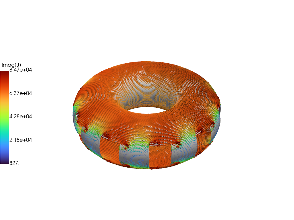
The resulting currents can be saved for plotting using tw_torus.save_current(). Here we save each of the five eigenvectors for visualization. Once all fields have been saved for plotting tw_torus.build_XDMF() to generate the XDMF descriptor files for plotting with VisIt of Paraview. This method also returns a XDMF_plot_file object, which can be used to read and interact with plot data in Python (see below).
Creating output files: oft_xdmf.XXXX.h5
  Removing old Xdmf files
    Removed 23 files
  Found Group: thincurr
    Found Mesh: icoils
    Found Mesh: smesh
Now we plot the current vectors on the plate showing the longest-lived eddy current structure, which corresponds to a large circulation on the plate. The XDMF_plot_file class provides functionality to work with the data stored in OFT plot files, including methods to generate information for 3D plotting in Python using pyvista.
Plotting data is always associated with a specific mesh, which is itself associated with a physics group. In this case ThinCurr is the physics group and the data we are interested in is stored on the surface mesh smesh. The plot_data['ThinCurr']['smesh'] is a XDMF_plot_mesh object with further functionality for accessing data.
To plot the first eigenvector we first get the pyvista plotting grid using get_pyvista_grid() and then retrieve the vertex-centered field (J_01_v) using get_field()
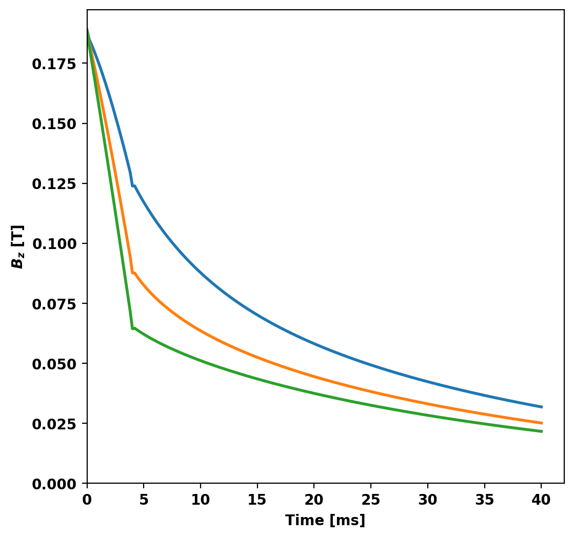
With the model fully defined we can now use run_td() to perform a time-domain simulation. In this case we simulate 40 ms using a timestep of 0.2 ms (200 steps). We also specify the current in the single I-coil defined in the XML input file as a function of time (coil_currs), where the first column specifies time points in ascending order and the remaining columns specify coil currents at each time point.
As we don't fully form the matrix with HODLR compression an iterative solver (Conjugate Gradient) is used on each time step. For performance considerations it is desirable to used the least restrictive convergence tolerance for this solver that provides the desired accuracy. This can be controlled using the lin_tol and lin_rtol arguments, which set absolute ( \(|E_i|_2 < \) lin_tol) and relative ( \(|E_i|_2/|E_0|_2 < \) lin_rtol) convergence criteria where \(|E_i|_2\) is the 2-norm of the solution error at the \(i\)-th iteration. In general, these parameters should be scanned for new cases to ensure the solutions are converged to within the desired accuracy.
Starting time-domain simulation
  timestep    time           sol_norm     nits    solver time
      10    2.000000E-03    2.2732E+01      28        0.14
      20    4.000000E-03    4.4119E+01      11        0.06
      30    6.000000E-03    4.2203E+01      11        0.06
      40    8.000000E-03    3.9905E+01      10        0.05
      50    1.000000E-02    3.7769E+01      10        0.05
      60    1.200000E-02    3.5770E+01      10        0.05
      70    1.400000E-02    3.3891E+01       9        0.05
      80    1.600000E-02    3.2121E+01       9        0.05
      90    1.800000E-02    3.0450E+01       9        0.05
     100    2.000000E-02    2.8873E+01       9        0.05
     110    2.200000E-02    2.7381E+01       9        0.05
     120    2.400000E-02    2.5970E+01       9        0.05
     130    2.600000E-02    2.4635E+01       9        0.05
     140    2.800000E-02    2.3370E+01       8        0.04
     150    3.000000E-02    2.2173E+01       8        0.04
     160    3.200000E-02    2.1038E+01       8        0.04
     170    3.400000E-02    1.9963E+01       8        0.04
     180    3.600000E-02    1.8944E+01       8        0.04
     190    3.800000E-02    1.7979E+01       7        0.04
     200    4.000000E-02    1.7063E+01       7        0.04
 Building block low rank magnetic field operator
   Building hole and Vcoil columns
   Building diagonal blocks
     10%
     20%
     30%
     40%
     50%
     60%
     70%
     80%
     90%
   Building off-diagonal blocks using ACA+
     10%
     20%
     30%
     40%
     50%
     60%
     70%
     80%
     90%
     Compression ratio:   7.1%  ( 1.06E+08/ 1.49E+09)
     Time =  1m 57s
   Saving HODLR matrix from file: HODLR_B.save
Post-processing time-domain simulation

Creating output files: oft_xdmf.XXXX.h5
  Removing old Xdmf files
    Removed 2 files
  Found Group: thincurr
    Found Mesh: icoils
    Found Mesh: smesh
OFT History file: floops.hist
  Number of fields = 4
  Number of entries = 201

  Fields:
    time: Simulation time [s] (d1)
    Bz_1: No description (d1)
    Bz_2: No description (d1)
    Bz_3: No description (d1)