|
The Open FUSION Toolkit 26.6
An open-source framework for fusion and plasma science and engineering
|
Loading...
Searching...
No Matches
|
The Open FUSION Toolkit 26.6
An open-source framework for fusion and plasma science and engineering
|
In this example we demonstrate how to build a reduced model from a large ThinCurr model and apply that model to time-domain simulations.
To load the ThinCurr python module we need to tell python where to the module is located. This can be done either through the PYTHONPATH environment variable or within a script using sys.path.append() as below, where we look for the environement variable OFT_ROOTPATH to provide the path to where the OpenFUSIONToolkit is installed (/Applications/OFT for binaries on macOS).
We now create a OFT_env instance for execution using four threads and a ThinCurr instance that utilizes that execution environment.
Once created, we setup the model from an existing HDF5 and XML mesh definition using setup_model().
We also initialize I/O for this model using setup_io() to enable output of plotting files for 3D visualization in VisIt, Paraview, or using pyvista below.
#----------------------------------------------
             ____  ____________
            / __ \/ ____/_  __/
           / / / / /_    / /
          / /_/ / __/   / /
          \____/_/     /_/

Base release:        v1.0.0-beta7
Development branch:  release_26_06
Revision id:         978c4b9f

Parallelization Info:
  Not compiled with MPI
  # of OpenMP threads =    4

Linear Algebra backend: native

#----------------------------------------------


Creating thin-wall model
  No V(t) driver coils found
  Loading I(t) driver coils
    Masked      0 coils from sensors
  Building holes

  Loading region surface resistivity:
     1  1.2570E-05

  Setup complete:
    # of points    =        22580
    # of edges     =        67150
    # of cells     =        44560
    # of holes     =           11
    # of closures  =            0
    # of Vcoils    =            0
    # of Icoils    =            1
To visualize the results we define three Mirnov sensors spanning one port period, just outside the torus. While every sensor in ThinCurr is a flux loop, helper classes for defining specific types of common sensors (eg. circular loop or Mirnovs) are available in OpenFUSIONToolkit.ThinCurr.sensor, which also contains the save_sensors() function for saving this information to a ThinCurr-compatible file format.
After defining the sensors we use compute_Msensor() to setup the sensors and compute mutual matrices between the sensors and the model (Msensor) and the sensors and Icoils (Msc).
Loading sensor information
  Loading flux loops from file: floops.loc
    # of floops =
␃
Building element->sensor inductance matrix
  Time =  0s
Building coil->sensor inductance matrix
  Time =  0s
With the model setup, we can now compute the self-inductance matrix using HODLR. When HODLR is used the result is a pointer to the Fortran operator, which is stored at tw_torus.Lmat_hodlr. As in any other case, by default, the resistivity matrix is not moved to python as it is sparse and converting to dense representation would require an increase in memory. These matrices correspond to the \(\textrm{L}\) and \(\textrm{R}\) matrices for the physical system
\(\textrm{L} \frac{\partial I}{\partial t} + \textrm{R} I = V\)
Building coil<->element inductance matrices
  Time =  0s
 Partitioning grid for block low rank compressed operators
   nBlocks =                  32
   Avg block size =          686
   # of SVD =                167
   # of ACA =                161

 Building block low rank inductance operator
   Building hole and Vcoil columns
   Reading HODLR matrix from file: HOLDR_L.save
   Building diagonal blocks
     10%
     20%
     30%
     40%
     50%
     60%
     70%
     80%
     90%
   Building off-diagonal blocks using ACA+
     10%
     20%
     30%
     40%
     50%
     60%
     70%
     80%
     90%
     Compression ratio:   6.1%  ( 2.94E+07/ 4.82E+08)
     Time =  3s
Building resistivity matrix
With \(\textrm{L}\) and \(\textrm{R}\) matrices we can now compute the eigenvalues and eigenvectors of the system \(\textrm{L} I = \lambda \textrm{R} I\), where the eigenvalues \(\lambda = \tau_{L/R}\) are the decay time-constants of the current distribution corresponding to each eigenvector.
Starting eigenvalue solve (ARPACK)
  Time =   1.7764E+00
  Eigenvalues
      3.880353E-02
      2.312241E-02
      2.312132E-02
      2.144471E-02
      2.060557E-02
With the model fully defined we can now use run_td() to perform a time-domain simulation. In this case we simulate 40 ms using a timestep of 0.2 ms (200 steps). We also specify the current in the single I-coil defined in the XML input file as a function of time (coil_currs), where the first column specifies time points in ascending order and the remaining columns specify coil currents at each time point.
As we don't fully form the matrix with HODLR compression an iterative solver (Conjugate Gradient) is used on each time step. For performance considerations it is desirable to used the least restrictive convergence tolerance for this solver that provides the desired accuracy. This can be controlled using the lin_tol and lin_rtol arguments, which set absolute ( \(|E_i|_2 < \) lin_tol) and relative ( \(|E_i|_2/|E_0|_2 < \) lin_rtol) convergence criteria where \(|E_i|_2\) is the 2-norm of the solution error at the \(i\)-th iteration. In general, these parameters should be scanned for new cases to ensure the solutions are converged to within the desired accuracy.
Starting time-domain simulation
  timestep    time           sol_norm     nits    solver time
      10    2.000000E-03    2.2732E+01      28        0.14
      20    4.000000E-03    4.4119E+01      11        0.06
      30    6.000000E-03    4.2203E+01      11        0.06
      40    8.000000E-03    3.9905E+01      10        0.05
      50    1.000000E-02    3.7769E+01      10        0.05
      60    1.200000E-02    3.5770E+01      10        0.05
      70    1.400000E-02    3.3891E+01       9        0.05
      80    1.600000E-02    3.2121E+01       9        0.05
      90    1.800000E-02    3.0450E+01       9        0.05
     100    2.000000E-02    2.8873E+01       9        0.05
     110    2.200000E-02    2.7381E+01       9        0.05
     120    2.400000E-02    2.5970E+01       9        0.05
     130    2.600000E-02    2.4635E+01       9        0.05
     140    2.800000E-02    2.3370E+01       8        0.05
     150    3.000000E-02    2.2173E+01       8        0.05
     160    3.200000E-02    2.1038E+01       8        0.05
     170    3.400000E-02    1.9963E+01       8        0.05
     180    3.600000E-02    1.8944E+01       8        0.05
     190    3.800000E-02    1.7979E+01       7        0.04
     200    4.000000E-02    1.7063E+01       7        0.04
 Building block low rank magnetic field operator
   Building hole and Vcoil columns
   Reading HODLR matrix from file: HODLR_B.save
   Building diagonal blocks
     10%
     20%
     30%
     40%
     50%
     60%
     70%
     80%
     90%
   Building off-diagonal blocks using ACA+
     10%
     20%
     30%
     40%
     50%
     60%
     70%
     80%
     90%
     Compression ratio:   7.1%  ( 1.05E+08/ 1.49E+09)
     Time =  2s
Post-processing time-domain simulation

Creating output files: oft_xdmf.XXXX.h5
  Removing old Xdmf files
    Removed 23 files
  Found Group: thincurr
    Found Mesh: icoils
    Found Mesh: smesh
OFT History file: floops.hist
  Number of fields = 4
  Number of entries = 201

  Fields:
    time: Simulation time [s] (d1)
    Bz_1: No description (d1)
    Bz_2: No description (d1)
    Bz_3: No description (d1)
In addition to HODLR, we can also explicitly reduce the model's size by projecting onto a fixed set of current strucutures using build_reduced_model(). In this case we use the 25 eigenvalues computed above, which will result in a system that reasonably matches slow dynamics with characterisitic times longer than the fastest eigenvalue.
After building the reduced system was can compare the eigenvalues of the original system to show that the characteristic timescales are maintained.
  Reduced      Original     (% Error )
  3.8804E+01   3.8804E+01   (4.32E-09)
  2.3122E+01   2.3122E+01   (2.15E-09)
  2.3121E+01   2.3121E+01   (1.10E-09)
  2.1445E+01   2.1445E+01   (1.91E-08)
  2.0606E+01   2.0606E+01   (1.20E-09)
   ...          ...          ...
  1.8735E+01   1.8735E+01   (4.89E-09)
  5.7417E+00   5.7417E+00   (3.01E-09)
  5.6741E+00   5.6741E+00   (2.51E-09)
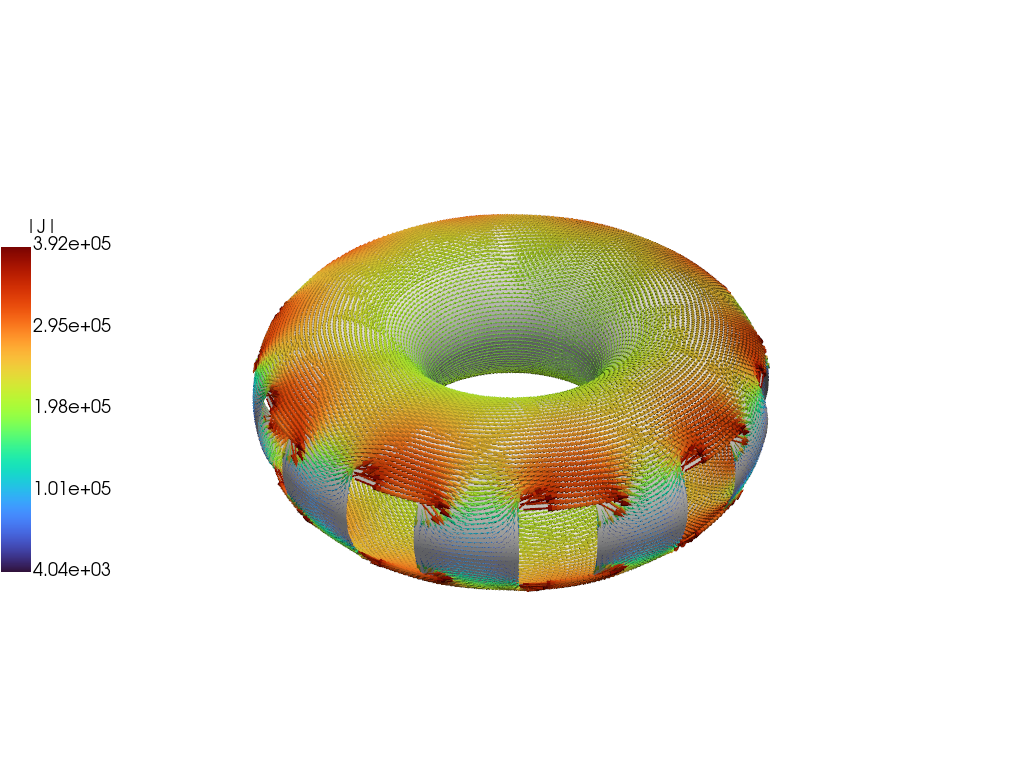
We can also plot the current distributions for the eigenmodes to show that they have the same structure as the original model.
Timestep 0   0.0000E+00   0.0000E+00
Timestep 10   2.0000E-03   3.1344E+00
Timestep 20   4.0000E-03   6.0592E+00
Timestep 30   6.0000E-03   5.7573E+00
Timestep 40   8.0000E-03   5.4154E+00
Timestep 50   1.0000E-02   5.1068E+00
Timestep 60   1.2000E-02   4.8245E+00
Timestep 70   1.4000E-02   4.5637E+00
Timestep 80   1.6000E-02   4.3210E+00
Timestep 90   1.8000E-02   4.0941E+00
Timestep 100   2.0000E-02   3.8811E+00
Timestep 110   2.2000E-02   3.6806E+00
Timestep 120   2.4000E-02   3.4915E+00
Timestep 130   2.6000E-02   3.3129E+00
Timestep 140   2.8000E-02   3.1440E+00
Timestep 150   3.0000E-02   2.9841E+00
Timestep 160   3.2000E-02   2.8327E+00
Timestep 170   3.4000E-02   2.6892E+00
Timestep 180   3.6000E-02   2.5531E+00
Timestep 190   3.8000E-02   2.4241E+00
Timestep 200   4.0000E-02   2.3017E+00
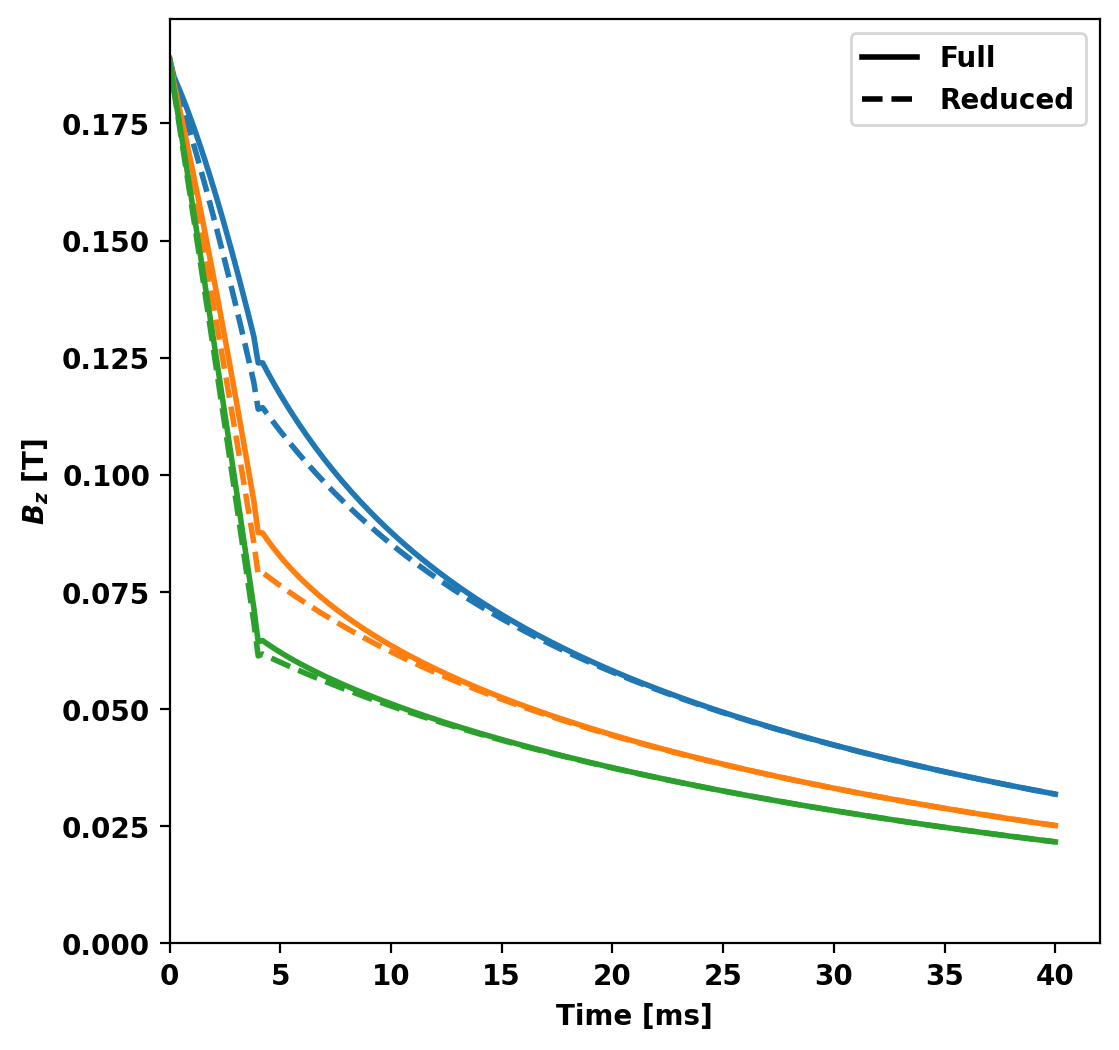
Now we compare the probe signals from full and reduced models, noting good agreement overall with some discrepancy early in time with the results converging at later times.
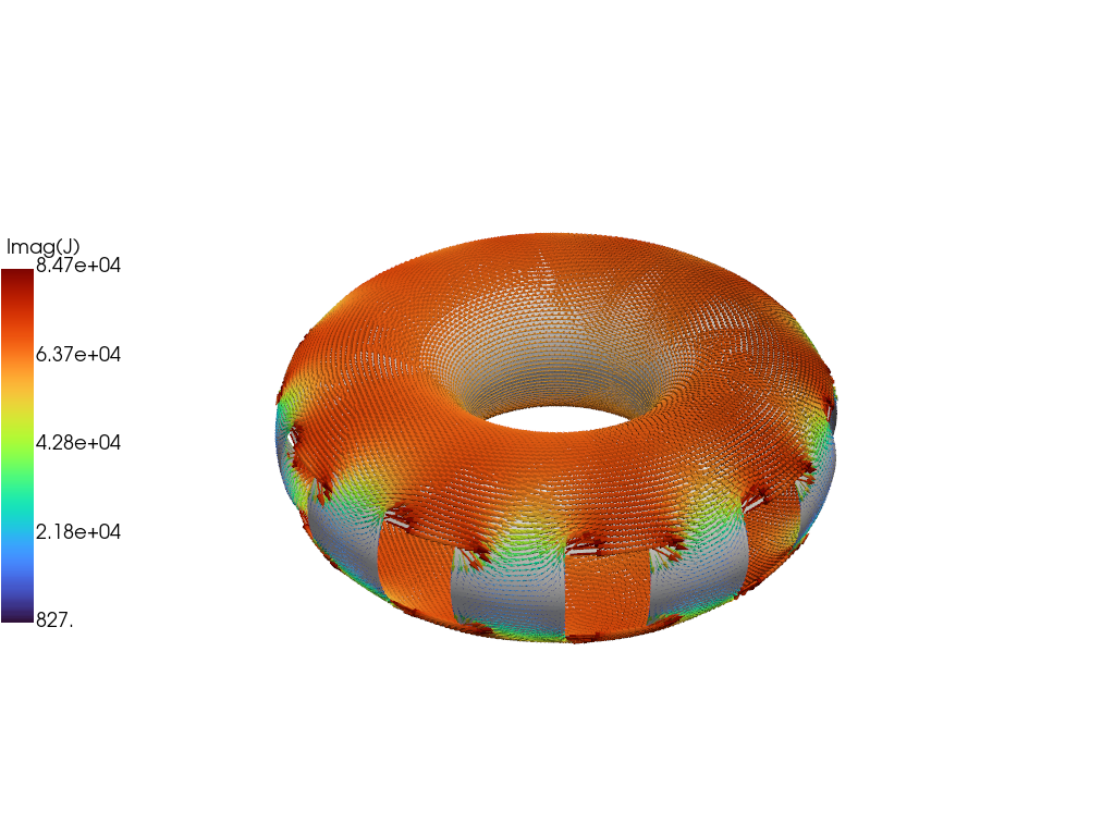
We can plot the current distributions for the eigenmodes to show that they have nearly the same structure and time-dependence as the full model. Below comparison is performed at \(t = 20\) ms showing good agreement, which should only improve at later times.
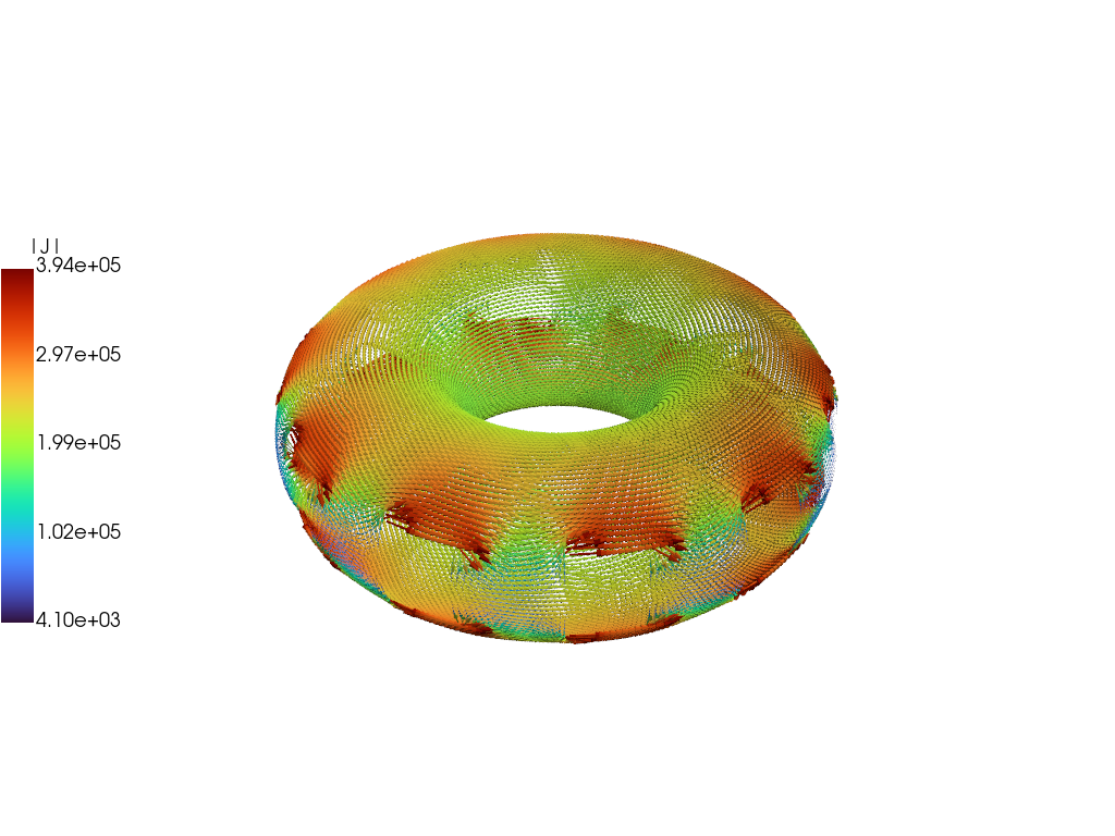
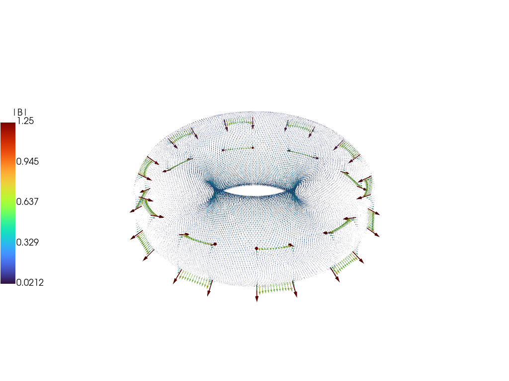
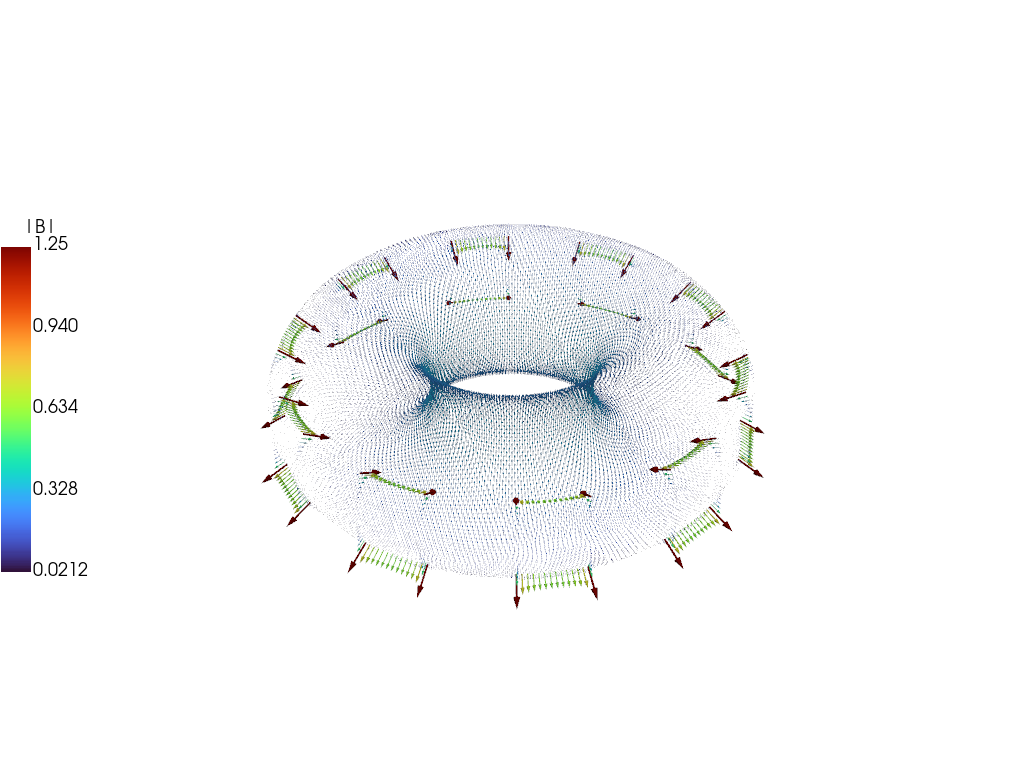
As with the current we can also compare the magnetic field between the full simulation and the reduced model, showing excellent visual agreement at \(t = 20\) ms.
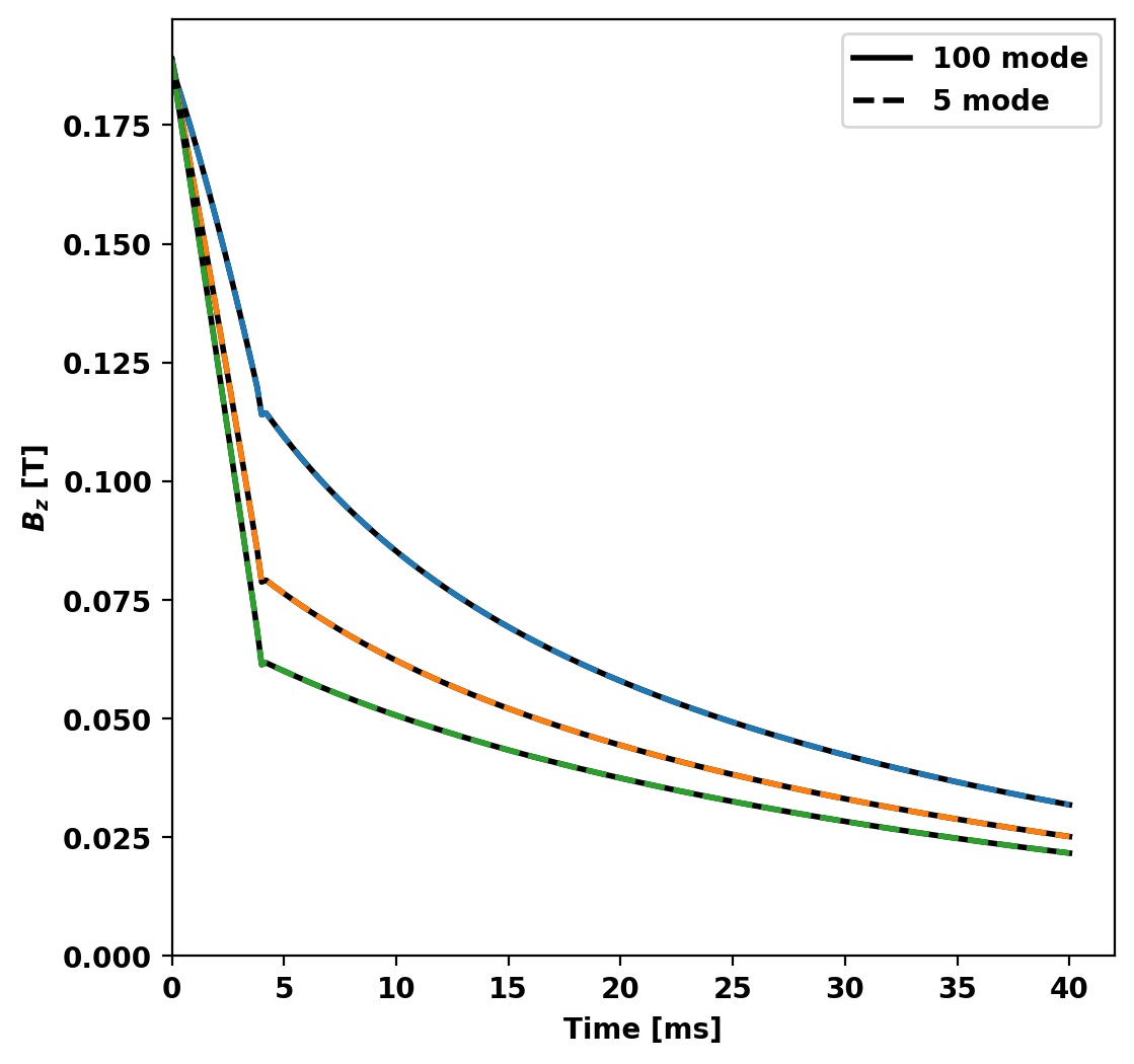
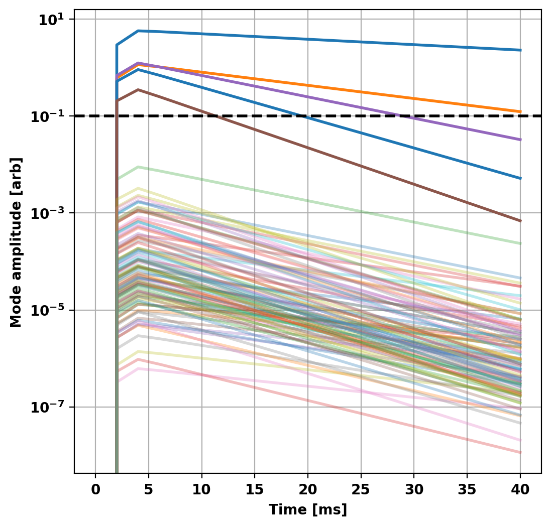
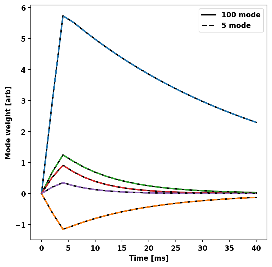
To further reduce the model we can look at the output of the previous to determine which modes in the basis set are active in the chosen simulation. In this case, the vast majority of the energy in the system is contained in only the first 5 modes.
This makes sense as all the sources driving our system are axisymmetric (single circular current filament) and as a result we expect all the eigenstructures with toroidal mode number greater than zero to have very little coupling to this structure (ideally zero). Additionally, as the L/R system results in orthogonal eigenvectors we don't expect any coupling between modes themselves. This can be seen as all modes decay exponentially (linear on semilog plot) after the driving voltage drops to zero.
We now repeat the eigenvalue and time-domain solves from above with the further reduced model.
  Reduced      Original     (% Error )
  3.8804E+01   3.8804E+01   (4.32E-09)
  1.6008E+01   1.6008E+01   (2.66E-09)
  9.8463E+00   9.8463E+00   (1.83E-09)
  6.9472E+00   6.9472E+00   (1.86E-09)
  5.7673E+00   5.7673E+00   (7.25E-10)
Timestep 0   0.0000E+00   0.0000E+00
Timestep 10   2.0000E-03   3.1344E+00
Timestep 20   4.0000E-03   6.0592E+00
Timestep 30   6.0000E-03   5.7573E+00
Timestep 40   8.0000E-03   5.4154E+00
Timestep 50   1.0000E-02   5.1068E+00
Timestep 60   1.2000E-02   4.8245E+00
Timestep 70   1.4000E-02   4.5637E+00
Timestep 80   1.6000E-02   4.3210E+00
Timestep 90   1.8000E-02   4.0941E+00
Timestep 100   2.0000E-02   3.8811E+00
Timestep 110   2.2000E-02   3.6806E+00
Timestep 120   2.4000E-02   3.4915E+00
Timestep 130   2.6000E-02   3.3129E+00
Timestep 140   2.8000E-02   3.1440E+00
Timestep 150   3.0000E-02   2.9841E+00
Timestep 160   3.2000E-02   2.8327E+00
Timestep 170   3.4000E-02   2.6892E+00
Timestep 180   3.6000E-02   2.5531E+00
Timestep 190   3.8000E-02   2.4241E+00
Timestep 200   4.0000E-02   2.3017E+00
First we compare the amplitude of each component (basis weight) of the two reduced models in time to show that they have the same behavior even with fewer modes in the system.
Now we compare the probe signals from the two reduced models showing that the results overlay eachother.