|
The Open FUSION Toolkit 26.6
An open-source framework for fusion and plasma science and engineering
|
Loading...
Searching...
No Matches
|
The Open FUSION Toolkit 26.6
An open-source framework for fusion and plasma science and engineering
|
In this example we demonstrate how to compute a current potential from a given B-norm on a toroidal surface. This has application to compute eddy current and sensor reponse to plasma modes.
To load the ThinCurr python module we need to tell python where to the module is located. This can be done either through the PYTHONPATH environment variable or within a script using sys.path.append() as below, where we look for the environement variable OFT_ROOTPATH to provide the path to where the OpenFUSIONToolkit is installed (/Applications/OFT for binaries on macOS).
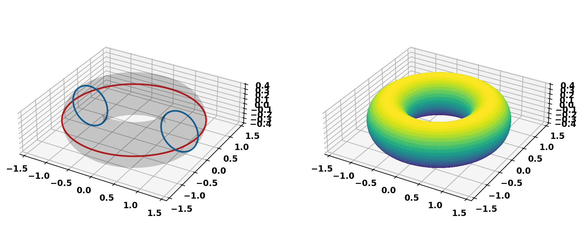
In most cases the mode will be imported and/or converted from another tool (eg. DCON). However, in this case we will generate a simple mode shape with fixed toroidal and poloidal mode number for a simple torus. Using a simple helper function we define an n=2, m=3 mode on an R=1.0 m, a=0.4 m torus.
We can now create a ThinCurr model from the mode definition file by using build_torus_bnorm_grid() to build a uniform grid over one toroidal field period and ThinCurr_periodic_toroid, which provides functionality for working with toroidally periodic meshes. The result is a ThinCurr_periodic_toroid object (plasma_mode) and the normal field at each mesh vertex for the Real and Imaginary components of the mode (bnorm).
Loading toroidal plasma mode
  filename = tCurr_mode.dat
  N        = 2
  # of pts = 200
  R0       = (1.0000E+00, -1.7087E-17)
  Mode pair sums -7.6050E-15 -2.9976E-15
Saving mesh: thincurr_mode.h5
We now create a OFT_env instance for execution using four threads and a ThinCurr instance that utilizes that execution environment. Once created, we setup the model from an existing HDF5 and XML mesh definition using setup_model().
We also initialize I/O for this model using setup_io() to enable output of plotting files for 3D visualization in VisIt or Paraview.
In this case we specify a plasma directory to use for saving I/O files to keep things separate for the other cases to be run in ThinCurr Python Example: Compute frequency-response in a torus.
#----------------------------------------------
             ____  ____________
            / __ \/ ____/_  __/
           / / / / /_    / /
          / /_/ / __/   / /
          \____/_/     /_/

Base release:        v1.0.0-beta7
Development branch:  release_26_06
Revision id:         978c4b9f

Parallelization Info:
  Not compiled with MPI
  # of OpenMP threads =    4

Linear Algebra backend: native

#----------------------------------------------


Creating thin-wall model
  No V(t) driver coils found
  No I(t) driver coils found
  Building holes

  Setup complete:
    # of points    =         6320
    # of edges     =        18960
    # of cells     =        12640
    # of holes     =            3
    # of closures  =            2
    # of Vcoils    =            0
    # of Icoils    =            0


WARNING: No "thincurr" XML node specified. Ignore this warning if an XML node does not need to be specified.
With the model setup, we can now compute the self-inductance matrix. A numpy version of the self-inductance matrix will be stored at tw_plate.Lmat. For this case we will use the self-inductance to convert between the surface flux \(\Phi\) corresponding to the normal field computed above (bnorm) and an equivalent surface current
\(\textrm{L} I = \Phi\)
condense_matrix() is then used collapse periodic copies into a final inductance matrix for the DOF of the periodic system.
Finally, we compute \(\textrm{L}^{-1}\).
Building element<->element self inductance matrix
  Time =  8s
Now we can compute the equivalent currents for the Real and Imaginary component of normal field \(B_n\) from above. To do this we need to convert to flux \(\Phi\) by scaling the field by the area of each vertex using scale_va(). As scale_va() acts on all vertices in the grid the plasma_mode.r_map index array is used to map to/from the full and single period spaces.
When computing the current density from the flux nodes_to_unique() is used to map from node points to unique DOFs by adding the toroidal and poloidal holes and removing closure elements.
Finally, when saving the current the output it expanded to the model size using expand_vector().
Creating output files: oft_xdmf.XXXX.h5
  Removing old Xdmf files
    Removed 0 files
  Found Group: thincurr
    Found Mesh: smesh
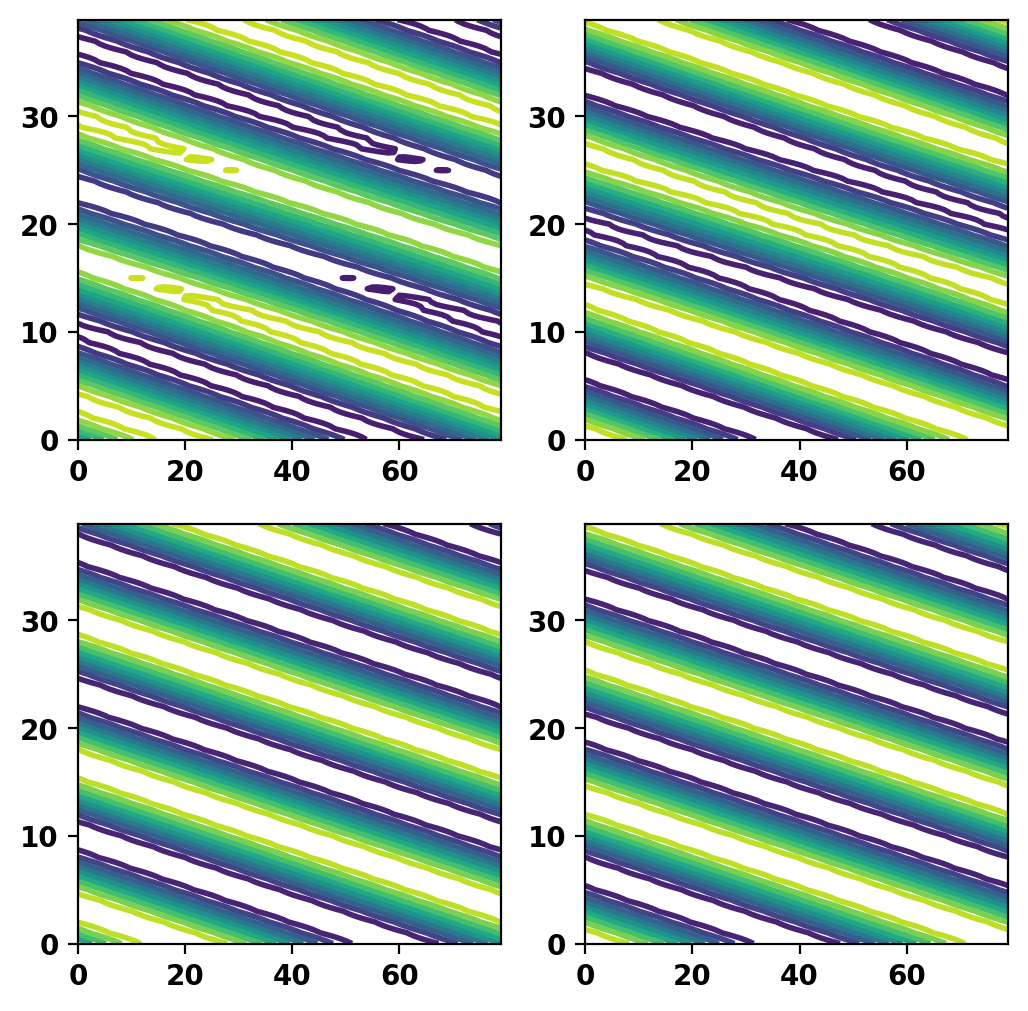
We now plot the resulting current potential (top) and mode shape (bottom) over a single toroidal mode period to show how the fields are related and ensure no errors. The helper method unique_to_nodes_2D() is provided to map between unique DOF and vertices over a single field period, which are then mapped to a uniform 2D grid.
Finally we save the currents to the model file as a "driver" to utilize in frequency response calculations in ThinCurr Python Example: Compute frequency-response in a torus.