|
The Open FUSION Toolkit 26.6
An open-source framework for fusion and plasma science and engineering
|
Loading...
Searching...
No Matches
|
The Open FUSION Toolkit 26.6
An open-source framework for fusion and plasma science and engineering
|
In this example we demonstrate how to perform a time-domain simulation for a model driven by the plasma mode computed in ThinCurr Python Example: Compute current potential from B-norm.
To load the ThinCurr python module we need to tell python where to the module is located. This can be done either through the PYTHONPATH environment variable or within a script using sys.path.append() as below, where we look for the environement variable OFT_ROOTPATH to provide the path to where the OpenFUSIONToolkit is installed (/Applications/OFT for binaries on macOS).
We now create a OFT_env instance for execution using four threads and a ThinCurr instance that utilizes that execution environment. Once created, we setup the model from an existing HDF5 and XML mesh definition using setup_model().
We also initialize I/O for this model using setup_io() to enable output of plotting files for 3D visualization in VisIt, Paraview, or using pyvista below.
#----------------------------------------------
             ____  ____________
            / __ \/ ____/_  __/
           / / / / /_    / /
          / /_/ / __/   / /
          \____/_/     /_/

Base release:        v1.0.0-beta7
Development branch:  release_26_06
Revision id:         978c4b9f

Parallelization Info:
  Not compiled with MPI
  # of OpenMP threads =    2

Linear Algebra backend: native

#----------------------------------------------


Creating thin-wall model
  No V(t) driver coils found
  Loading I(t) driver coils
    Masked      0 coils from sensors
  Building holes

  Loading region surface resistivity:
     1  1.2570E-05

  Setup complete:
    # of points    =         2394
    # of edges     =         7182
    # of cells     =         4788
    # of holes     =            2
    # of closures  =            0
    # of Vcoils    =            0
    # of Icoils    =            1
Before running the main calculations we will also define some sensors to measure the magnetic field. In ThinCurr all sensors measure the flux passing through a 3D path of points, but there are several helper classes to define common sensors (eg. Poloidal flux and Mirnovs). Here we define two Mirnov sensors to measure the Z-component of the magnetic field 5 cm on either side of the torus. save_sensors() is then used to save the resulting sensor for later use.
After defining the sensors we use compute_Msensor() to setup the sensors and compute mutual matrices between the sensors and the model (Msensor) and the sensors and Icoils (Msc).
Loading sensor information
  Loading flux loops from file: floops.loc
    # of floops =
␄
Building element->sensor inductance matrix
  Time =  0s
Building coil->sensor inductance matrix
  Time =  0s
With the model setup, we can now compute the self-inductance and resistivity matrices. A numpy version of the self-inductance matrix will be stored at tw_torus.Lmat. By default the resistivity matrix is not moved to python as it is sparse and converting to dense representation would require an increase in memory. These matrices correspond to the \(\textrm{L}\) and \(\textrm{R}\) matrices for the physical system
\(\textrm{L} \frac{\partial I}{\partial t} + \textrm{R} I = V\)
Building coil<->element inductance matrices
  Time =  0s
Building element<->element self inductance matrix
  Time =  4s
Building resistivity matrix
We now create a second ThinCurr instance for the plasma mode utilizes the same execution environment as above. For this case we also load the plasma mode current patterns created in ThinCurr Python Example: Compute current potential from B-norm.
Creating thin-wall model
  No V(t) driver coils found
  No I(t) driver coils found
  Building holes

  Setup complete:
    # of points    =         6320
    # of edges     =        18960
    # of cells     =        12640
    # of holes     =            3
    # of closures  =            2
    # of Vcoils    =            0
    # of Icoils    =            0


WARNING: No "thincurr" XML node specified. Ignore this warning if an XML node does not need to be specified.
To use this current distribution we need the inductive coupling between the mode currents and the ThinCurr model of the wall (tw_wall). This can be done using cross_eval(), which in this case computes the flux through each element on tw_wall due to the currents specified by weights mode_drive corresponding to the model tw_mode. We also compute the coupling of the plasma mode to the sensors.
Loading sensor information
  Loading flux loops from file: floops.loc
    # of floops =
␄
Building element->sensor inductance matrix
  Time =  0s
Building coil->sensor inductance matrix
  No magnetic sensors or coils, skipping...
Applying MF element<->element inductance matrix
  Time = 20s
With the model fully defined we can now use run_td() to perform a time-domain simulation. In this case we simulate the mode with a growth rate of 2,000 1/s and a rotation frequency of 1 kHz for four periods using a timestep of 1/50 of the rotation period (200 steps). We also specify using a direct solver for the time-advance (direct=True).
The driver waveform is set by defining appropriate Sin/Cos scale functions for the driver basis functions (mode_driver) and their derivatives, which in turn correspond to scale factors for the current and voltage. These are then used to define a voltage source for the time-domain and the sensor signal produced by these currents, which are not directly included in the simulation.
Starting time-domain simulation
  timestep    time           sol_norm     nits    solver time
  Starting factorization
 Inverting real matrix
   Time =   0.13920099999999999
      10    2.000000E-04    3.9983E-07       1        0.00
      20    4.000000E-04    5.5657E-07       1        0.00
      30    6.000000E-04    1.0040E-06       1        0.00
      40    8.000000E-04    1.5244E-06       1        0.00
      50    1.000000E-03    1.1763E-06       1        0.00
      60    1.200000E-03    2.4465E-06       1        0.00
      70    1.400000E-03    1.9497E-06       1        0.00
      80    1.600000E-03    2.6759E-06       1        0.00
      90    1.800000E-03    3.4373E-06       1        0.00
     100    2.000000E-03    2.3643E-06       1        0.00
     110    2.200000E-03    4.4932E-06       1        0.00
     120    2.400000E-03    3.3429E-06       1        0.00
     130    2.600000E-03    4.3478E-06       1        0.00
     140    2.800000E-03    5.3502E-06       1        0.00
     150    3.000000E-03    3.5522E-06       1        0.00
     160    3.200000E-03    6.5399E-06       1        0.00
     170    3.400000E-03    4.7362E-06       1        0.00
     180    3.600000E-03    6.0197E-06       1        0.00
     190    3.800000E-03    7.2631E-06       1        0.00
     200    4.000000E-03    4.7400E-06       1        0.00
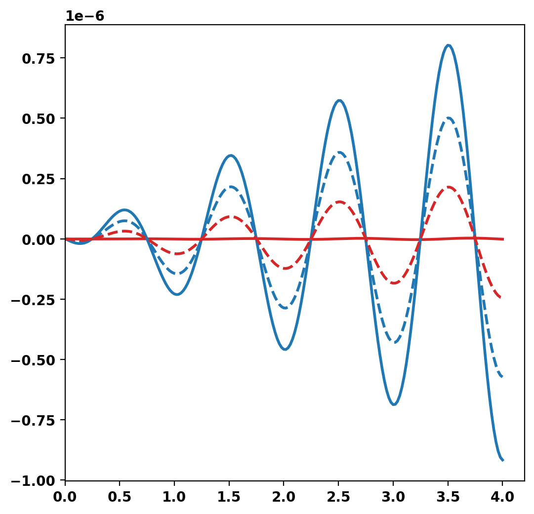
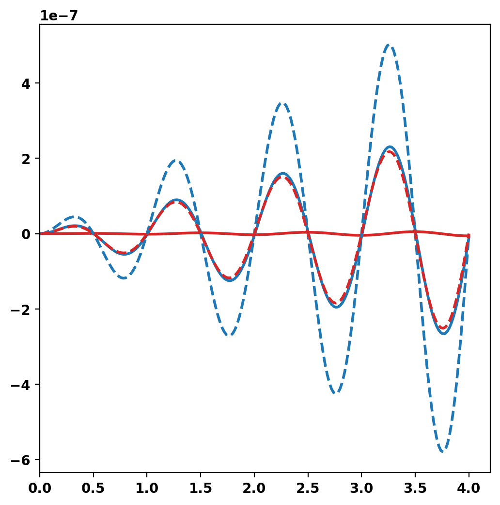
We can now plot the signals from the two flux loops defined above as a function of time. During the time-domain run this information is stored in OFT's binary history file format, which can be read using the histfile class. This class stores the resulting signals in a Python dict-like representation.
In the below plots the vacuum field (no eddy currents) is shown in the dashed lines and the full field is shown in the solid lines, where the external fields are suppressed by eddy currents and the internal tangential field (Bz_inner) is enhanced.
OFT History file: floops.hist
  Number of fields = 5
  Number of entries = 201

  Fields:
    time: Simulation time [s] (d1)
    Bz_inner: No description (d1)
    Bz_outer: No description (d1)
    Br_inner: No description (d1)
    Br_outer: No description (d1)
After completing the simulation we can generate plot files using tw_torus.plot_td(). Plot files are saved at a fixed timestep interval, specified by the nplot argument to run_td() with a default value of 10.
Once all fields have been saved for plotting tw_torus.build_XDMF() to generate the XDMF descriptor files for plotting with VisIt of Paraview. This method also returns a XDMF_plot_file object, which can be used to read and interact with plot data in Python (see below).
Post-processing time-domain simulation

Creating output files: oft_xdmf.XXXX.h5
  Removing old Xdmf files
    Removed 2 files
  Found Group: thincurr
    Found Mesh: icoils
    Found Mesh: smesh
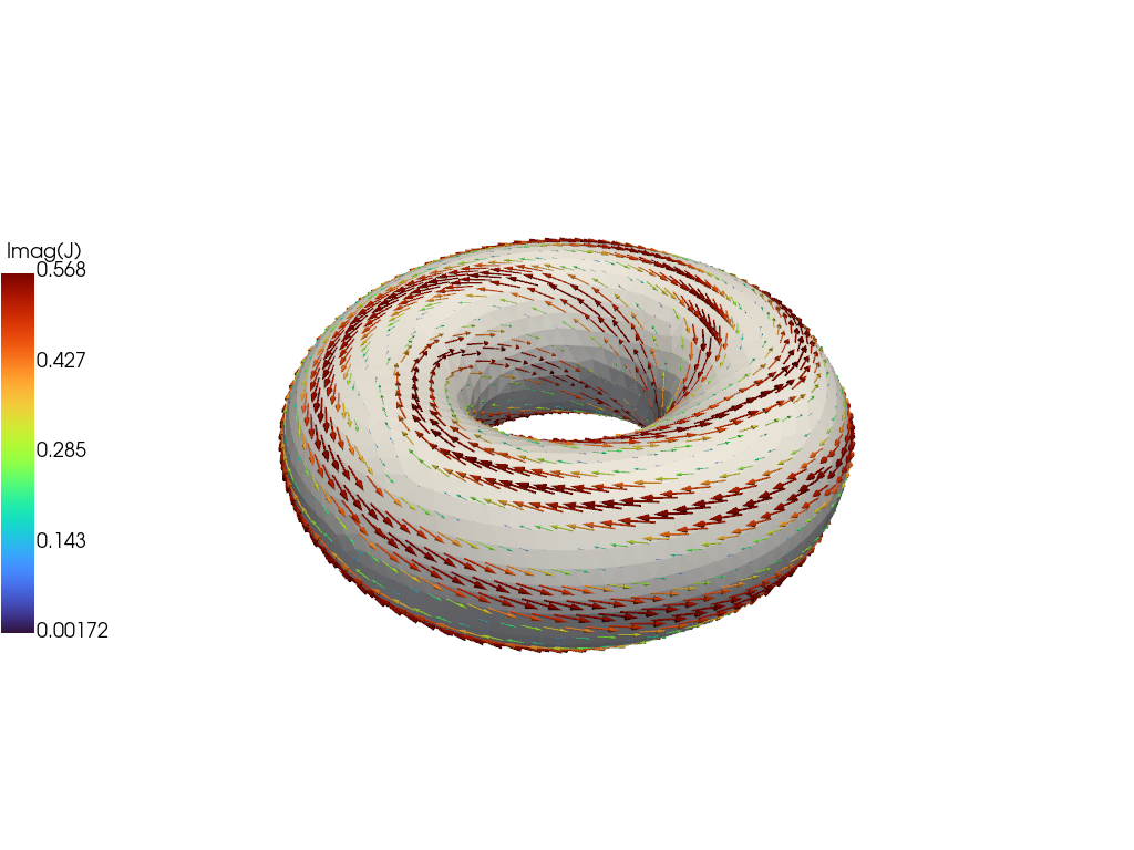
For demonstration purposes we now plot the the solution at the end of the driven phase using pyvista. We now use the plot_data object to generate a 3D plot of the current at t=2.E-3. For more information on the basic steps in this block see ThinCurr Python Example: Compute eigenstates in a plate