|
The Open FUSION Toolkit 26.6
An open-source framework for fusion and plasma science and engineering
|
Loading...
Searching...
No Matches
|
The Open FUSION Toolkit 26.6
An open-source framework for fusion and plasma science and engineering
|
In this example we demonstrate how to compute forces on a model using results of a time-domain simulation for a cylinder.
To load the ThinCurr python module we need to tell python where to the module is located. This can be done either through the PYTHONPATH environment variable or within a script using sys.path.append() as below, where we look for the environement variable OFT_ROOTPATH to provide the path to where the OpenFUSIONToolkit is installed (/Applications/OFT for binaries on macOS).
We now create a OFT_env instance for execution using two threads and a ThinCurr instance that utilizes that execution environment.
Once created, we setup the model from an existing HDF5 and XML mesh definition using setup_model(). For this model we have defined current jumpers using additional nodesets, which must be identified using the jumper_start argument (see ThinCurr Python Example: Time-domain simulation of a cylinder with jumpers for more information).
Finally, we initialize I/O for this model using setup_io() to enable output of plotting files for 3D visualization in VisIt, Paraview, or using pyvista below.
#----------------------------------------------
             ____  ____________
            / __ \/ ____/_  __/
           / / / / /_    / /
          / /_/ / __/   / /
          \____/_/     /_/

Base release:        v1.0.0-beta7
Development branch:  release_26_06
Revision id:         978c4b9f

Parallelization Info:
  Not compiled with MPI
  # of OpenMP threads =    2

Linear Algebra backend: native

#----------------------------------------------


Creating thin-wall model
  No V(t) driver coils found
  Loading I(t) driver coils
    Masked      0 coils from sensors
  Building holes

  Loading region surface resistivity:
     1  1.2570E-05

  Setup complete:
    # of points    =          782
    # of edges     =         2222
    # of cells     =         1440
    # of holes     =            1
    # of closures  =            0
    # of Vcoils    =            0
    # of Icoils    =            1
With the model setup, we can now compute the self-inductance and resistivity matrices. A numpy version of the self-inductance matrix will be stored at tw_plate.Lmat. By default the resistivity matrix is not moved to python as it is sparse and converting to dense representation would require an increase in memory. These matrices correspond to the \(\textrm{L}\) and \(\textrm{R}\) matrices for the physical system
\(\textrm{L} \frac{\partial I}{\partial t} + \textrm{R} I = V\)
Building coil<->element inductance matrices
  Time =  0s
Building element<->element self inductance matrix
  Time =  0s
Building resistivity matrix
With the model fully defined we can now use run_td() to perform a time-domain simulation. In this case we simulate 80 ms using a timestep of 0.2 ms (400 steps). We also specify using a direct solver for the time-advance (direct=True) and set the current in the single I-coil defined in the XML input file as a function of time (coil_currs), where the first column specifies time points in ascending order and the remaining columns specify coil currents at each time point.
Starting time-domain simulation
  timestep    time           sol_norm     nits    solver time
  Starting factorization
 Inverting real matrix
   Time =    6.9639999999999997E-003
      10    2.000000E-03    2.2123E-02       1        0.00
      20    4.000000E-03    4.2703E-02       1        0.00
      30    6.000000E-03    6.1352E-02       1        0.00
      40    8.000000E-03    7.8262E-02       1        0.00
      50    1.000000E-02    9.3611E-02       1        0.00
      60    1.200000E-02    1.0756E-01       1        0.00
      70    1.400000E-02    1.2025E-01       1        0.00
      80    1.600000E-02    1.3182E-01       1        0.00
      90    1.800000E-02    1.4237E-01       1        0.00
     100    2.000000E-02    1.5141E-01       1        0.00
     110    2.200000E-02    1.3822E-01       1        0.00
     120    2.400000E-02    1.2581E-01       1        0.00
     130    2.600000E-02    1.1464E-01       1        0.00
     140    2.800000E-02    1.0459E-01       1        0.00
     150    3.000000E-02    9.5529E-02       1        0.00
     160    3.200000E-02    8.7360E-02       1        0.00
     170    3.400000E-02    7.9981E-02       1        0.00
     180    3.600000E-02    7.3304E-02       1        0.00
     190    3.800000E-02    6.7253E-02       1        0.00
     200    4.000000E-02    6.1759E-02       1        0.00
     210    4.200000E-02    5.6763E-02       1        0.00
     220    4.400000E-02    5.2214E-02       1        0.00
     230    4.600000E-02    4.8065E-02       1        0.00
     240    4.800000E-02    4.4275E-02       1        0.00
     250    5.000000E-02    4.0810E-02       1        0.00
     260    5.200000E-02    3.7637E-02       1        0.00
     270    5.400000E-02    3.4729E-02       1        0.00
     280    5.600000E-02    3.2061E-02       1        0.00
     290    5.800000E-02    2.9610E-02       1        0.00
     300    6.000000E-02    2.7358E-02       1        0.00
     310    6.200000E-02    2.5286E-02       1        0.00
     320    6.400000E-02    2.3378E-02       1        0.00
     330    6.600000E-02    2.1621E-02       1        0.00
     340    6.800000E-02    2.0001E-02       1        0.00
     350    7.000000E-02    1.8507E-02       1        0.00
     360    7.200000E-02    1.7128E-02       1        0.00
     370    7.400000E-02    1.5855E-02       1        0.00
     380    7.600000E-02    1.4680E-02       1        0.00
     390    7.800000E-02    1.3594E-02       1        0.00
     400    8.000000E-02    1.2590E-02       1        0.00
After completing the simulation we can generate plot files using plot_td(). Plot files are saved at a fixed timestep interval, specified by the nplot argument to run_td(). By default this function only computes currents and sensor/jumper signal. To compute forces we also need the magnetic field, which can be computed by setting the argument compute_B=True.
Once all fields have been saved for plotting build_XDMF() to generate the XDMF descriptor files for plotting with VisIt of Paraview. This method also returns a XDMF_plot_file object, which can be used to read and interact with plot data in Python (see below).
Post-processing time-domain simulation
  Building element->element magnetic reconstruction operator
  Building vcoil->element magnetic reconstruction operator
  Building icoil->element magnetic reconstruction operator

Creating output files: oft_xdmf.XXXX.h5
  Removing old Xdmf files
    Removed 43 files
  Found Group: thincurr
    Found Mesh: icoils
    Found Mesh: smesh
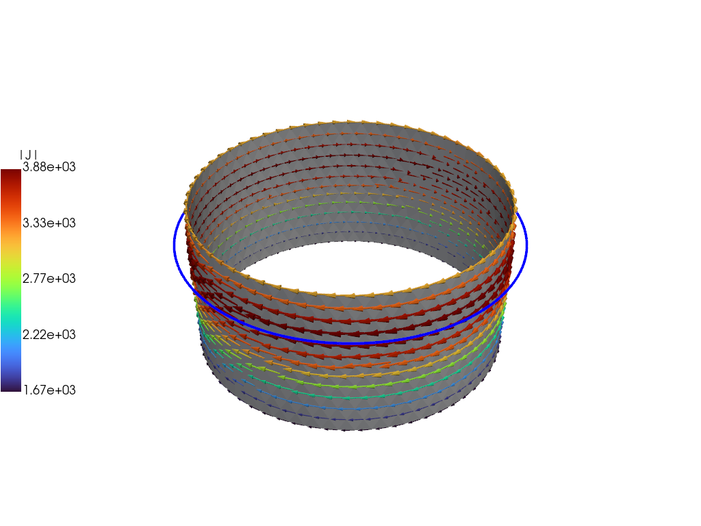
For demonstration purposes we now plot the the solution at the end of the driven phase using pyvista. We now use the plot_data object to generate a 3D plot of the current at t=2.E-2. For more information on the basic steps in this block see ThinCurr Python Example: Compute eigenstates in a plate
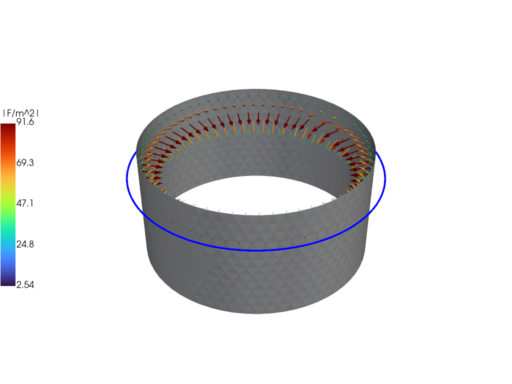
We can also plot the force distribution on the cylinder using both \(J\) and \(B\), which gives us the force per unit area over the surface of the cylinder.
We now demonstrate how to get the net force on the cylinder by integrating over the surface. To do this we first need some additional information, including the area of each cell (triangle) and the radial unit vector, which we will use to extract a hoop "force". For ThinCurr's triangular grid these can be readily computed from the information in the plotting mesh.
Then we define a helper function, which computes the desired net force on the cylinder from a cell-centered current density and vertex-centered magnetic field, which we will retrieve from the plot files. The function also supports an optional cell mask, which can be used to restrict the force calculation to specific areas (eg. one region or another in the mesh).
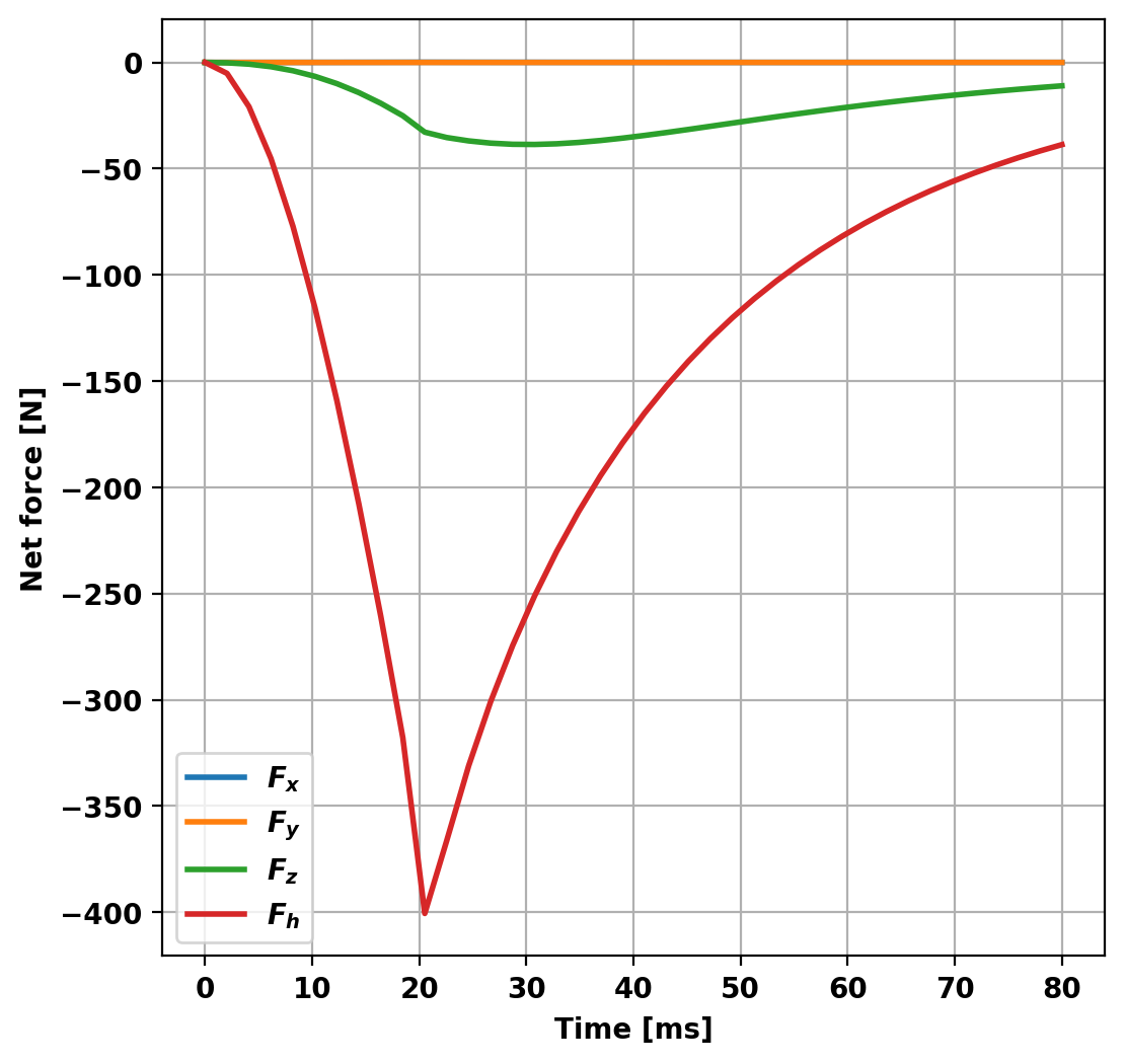
With this information and functionality we can now loop over the desired time points, computing the force at each time. The results show that a significant inward radial force and a downward vertical force, consistent with the physical arrangement of this test where the current in the coil ramps up in time acting to "crush" the cylinder and push it downward due to the vertical offset. Note that the net forces in the azimuthal plane (XY) are zero, so the hoop "force" is not a realy force per-se but instead a representation of the hoop stress that would be present.