Table of Contents
This example demonstrates the use of MUG to model self-heating of a spheromak in a unit cylinder. This process provides a simple example case illustrating the basic aspects of an MHD simulation, including: 1) Temperature dependent resistivity, 2) Anisotropic thermal conduction and 3) Ohmic and Viscous heating.
The dynamics in this example will be predominetly limited to heating. However, if the simulation is run long enough evolution of the equilibrium profile will be observed and eventual instability due to current peaking will occur.
Code Walk Through
The code consists of three basic sections, required imports and variable definitions, finite element setup, and system creation and solution.
Module Includes
The first thing that we must do is include the OFT modules which contain the required functions and variables. It is good practice to restrict the included elements to only those needed. This is done using the ONLY: clause to specifically include only certain definitions. The exceptions to this practice are the oft_local and oft_base modules, which contain a controlled set of commonly used elements that can be safely imported as a whole.
Local Variables
Next we define the local variables needed to initialize our case and run the time-dependent solve and post-processing.
OFT Initialization
See API Example 1: Helmholtz solve for a detailed description of calls in this section.
Perform post-processing
To visualize the solution fields once a simulation has completed the xmhd_plot subroutine is used. This subroutine steps through the restart files produced by xmhd_run and generates plot files, and optionally probe signals at evenly spaced points in time as specified in the input file, see xmhd_plot and Post-Processing options.
Computing Initial Conditions
For this simulation we only need the spheromak mode, which is the lowest force-free eignstate in this geometry. As a result the initial condition is stable to all types of mode activity.
As in MUG Example: Spheromak Tilt we must transform the gauge of the Taylor state solution to the appropriate magnetic field BCs. For more information on this see the description in Computing Initial Conditions of that example.
Now we set initial conditions for the simulation using the computed taylor state, flat temperature and density profiles and zero initial velocity. The lower bound for density (den_floor) and temperature (temp_floor) in the simulation are also set. These variables act to prevent very low density and negative temperature regions in the simulation. The scale factors for the velocity (vel_scale) and density (den_scale) evolution equations are also set. These variables are used to scale the corresponding rows in the non-linear and linear operators to provide even weighting in the residual calculations. In general these scale factors should be set to the order of magnitude expected for the corresponding variables, \( km/s \) and \( 10^{19} m^{-3} \) in this simulation.
Run Simulation
Finally, the simulation can be run using the driver routine for non-linear extended MHD (xmhd_run). This routine advances the solution in time with the physics specified in the input file, see the documentation for xmhd_run, and produces restart files that contain the solution at different times.
Several quantities are also recorded to a history file xmhd.hist during the simulation, including the toroidal current (where the symmetry axis is specified by xmhd_taxis). The data in the history file may be plotted using the script plot_mug_hist.py, which is located in src/utilities/scripts or python directories for the repository and an installation respectively.
- Note
- OFT plotting scripts require the python packages
numpyandmatplotlibas well as path access to the python modules provided inpythonfor installations orsrc/utilitiesin the repo.
To visualize the solution fields once a simulation has completed the xmhd_plot subroutine is used. This subroutine steps through the restart files produced by xmhd_run and generates plot files, and optionally probe signals at evenly spaced points in time as specified in the input file, see xmhd_plot.
Input file
Below is an input file which can be used with this example in a parallel environment. As with Example 5 this example should only be run with multiple processes. Some annotation of the options is provided inline below, for more information on the available options in the xmhd_options group see xmhd_plot.
&runtime_options
 ppn=1
 debug=0
/

&mesh_options
 meshname='test'
 cad_type=0
 nlevels=2
 nbase=1
 grid_order=2
 fix_boundary=T
/

&native_mesh_options
 filename='cyl_heat.h5'
/

&sph_heat_options
 order=3
 b0_scale=1.e-1
 n0=1.e19
 t0=6.
 plot_run=F
/

&xmhd_options
 xmhd_ohmic=T      ! Include Ohmic heating
 xmhd_visc_heat=T  ! Include viscous heating
 bbc='bc'          ! Perfectly-conducting BC for B-field
 vbc='all'         ! Zero-flow BC for velocity
 nbc='d'           ! Dirichlet BC for density
 tbc='d'           ! Dirichlet BC for temperature
 dt=2.e-7          ! Maximum time step
 eta=25.           ! Resistivity at reference temperature (Spitzer-like)
 eta_temp=6.       ! Reference temperature for resistivity
 nu_par=400.       ! Fluid viscosity
 d_dens=10.        ! Density diffusion
 kappa_par=1.E4    ! Parallel thermal conduction (fixed)
 kappa_perp=1.E2   ! Perpendicular thermal conduction (fixed)
 nsteps=2000       ! Number of time steps to take
 rst_freq=10       ! Restart file frequency
 lin_tol=1.E-9     ! Linear solver tolerance
 nl_tol=1.E-5      ! Non-linear solver tolerance
 xmhd_mfnk=T       ! Use matrix-free Jacobian operator
 rst_ind=0         ! Index of file to restart from (0 -> use subroutine arguments)
 ittarget=40       ! Target for # of linear iterations per time step
 mu_ion=2.         ! Ion mass (atomic units)
 xmhd_prefreq=20   ! Preconditioner update frequency
/
Solver specification
Time dependent MHD solvers are accelerated significantly by the use of a more sophisticated preconditioner than the default method. Below is an example oft_in.xml file that constructs an appropriate ILU(0) preconditioner. Currently, this preconditioner method is the suggested starting preconditioner for all time-dependent MHD solves.
This solver can be used by specifying both the FORTRAN input and XML input files to the executable as below.
~$ ./MUG_sph_heat oft.in oft_in.xml
Post-Processing options
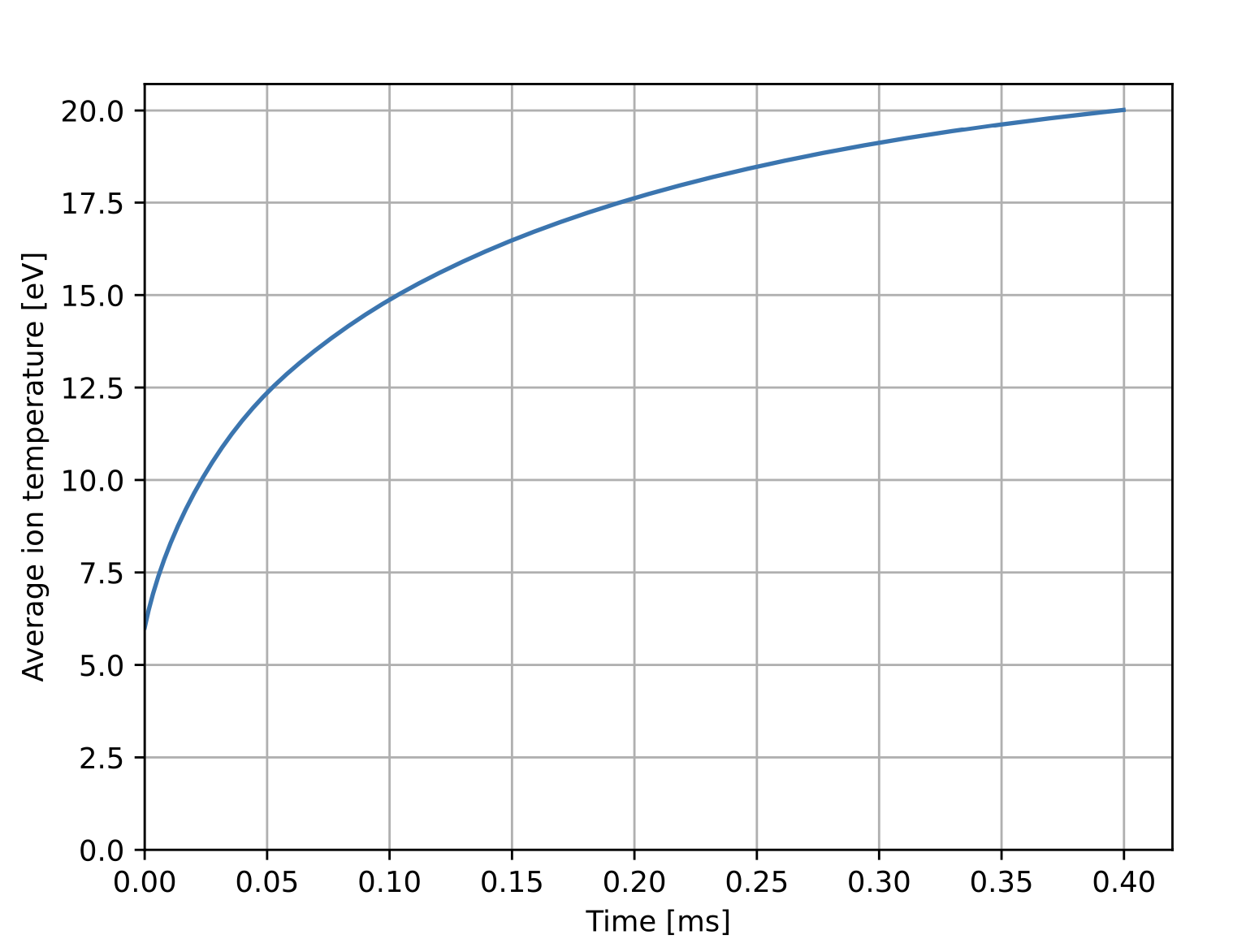
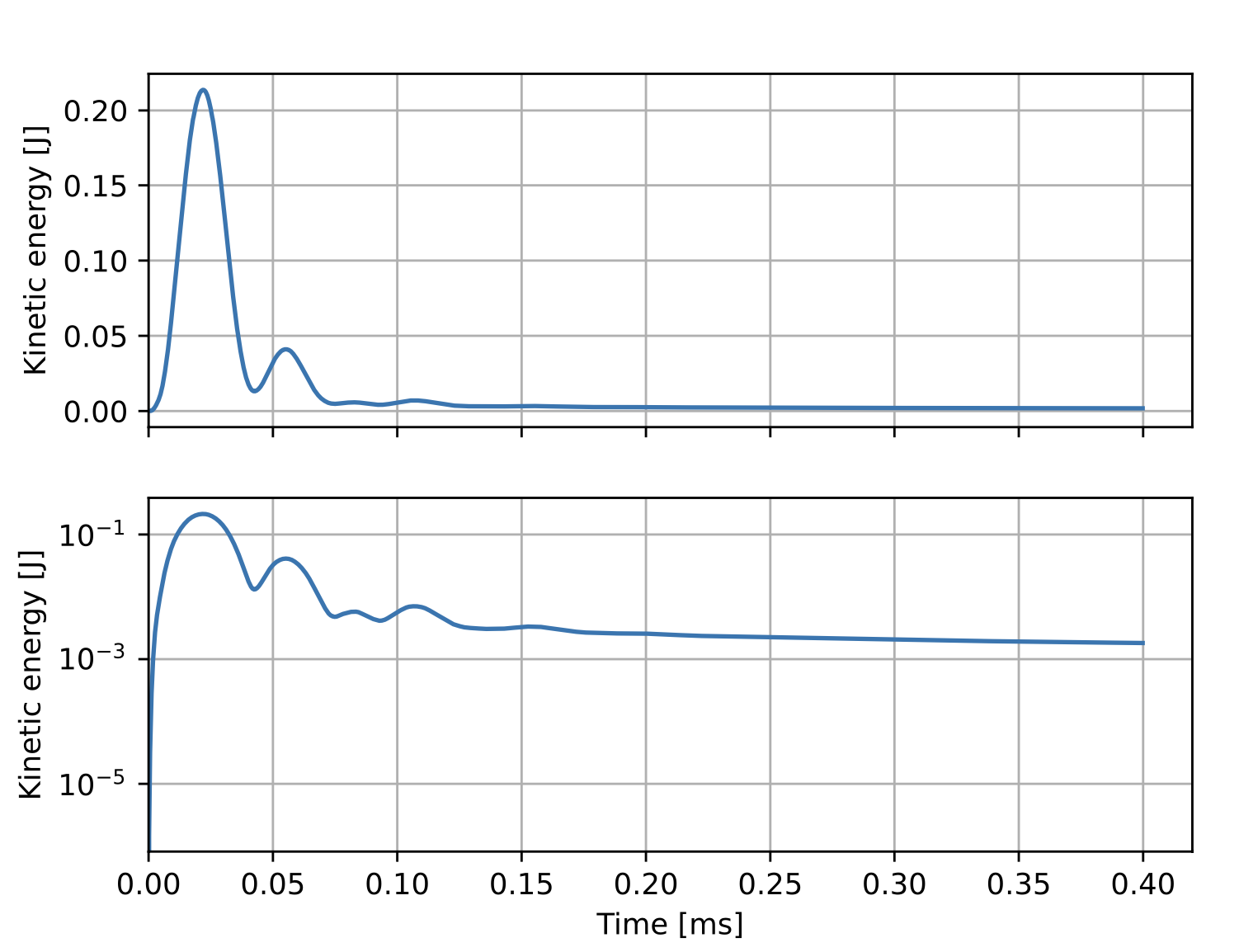
During the simulation the evolution of some global quantities is written to the history file xmhd.hist. A utility script (plot_mug_hist.py located in bin after installation) is included as part of OFT for plotting the signals in this file. This is useful for monitoring general progress of the simulation as well as numerical parameters like the iteration count and solver time. Using this script we can see the increase in the average temperature in time and a brief velocity transient early in time as equilibrium adjusts slightly to be consistent with the magnetic BCs used in the simulation.
~$ python plot_mug_hist.py xmhd.hist
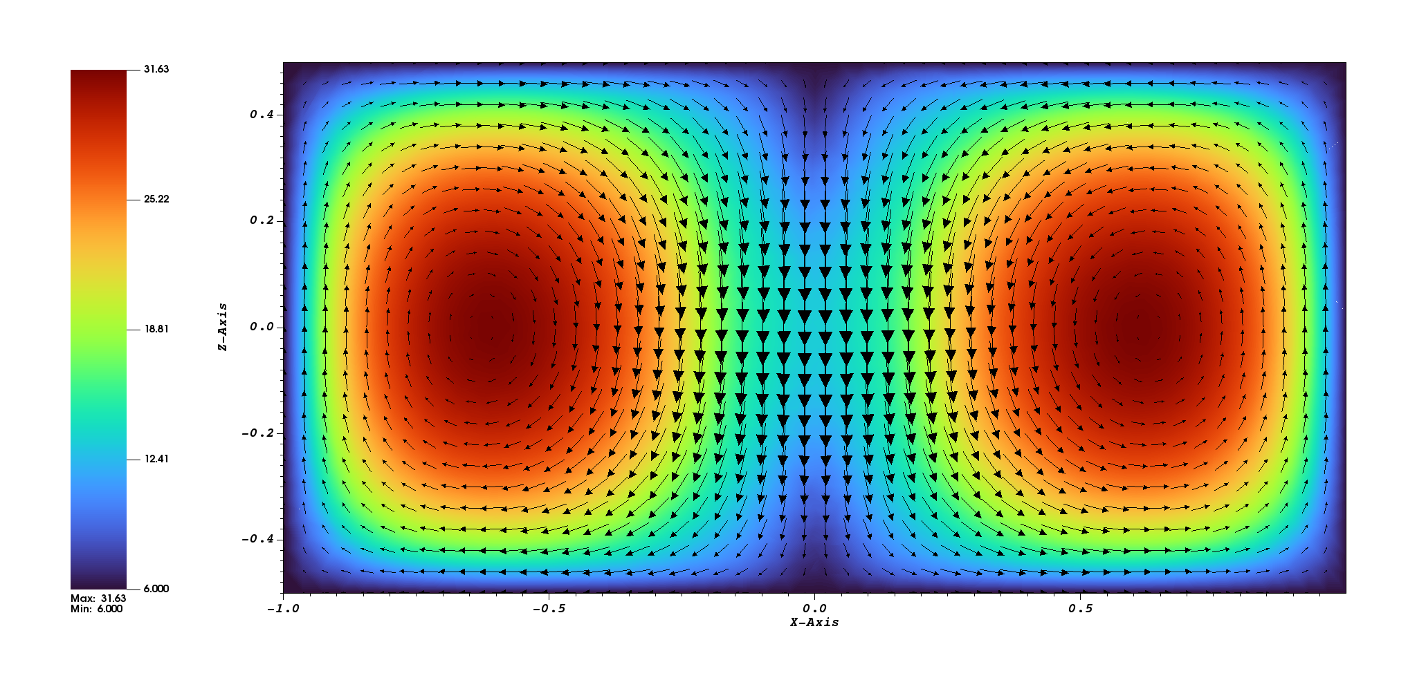
Creating plot files
To generate 3D plots, and perform additional diagnostic sampling (see oft_xmhd_probe), a plot run can be performed by setting plot_run=T in the sph_tilt_options input group, which calls xmhd_plot. With this option additional run time options are available in the xmhd_plot_options group that control how restart files are sampled for plotting.
&xmhd_plot_options
 t0=1.E-8
 dt=1.E-5
 rst_start=0
 rst_end=2000
/
Once the post-processing run is complete bin/build_xdmf.py can be used to generate *.xmf files that can be loaded by VisIt, ParaView, or other visualization programs.
Mesh Creation
A mesh file cyl_heat.h5 is provided with this example. Instructions to generate your own mesh for the geometry using CUBIT and GMSH.
Meshing with CUBIT
A suitable mesh for this example, with radius of 1m and height of 1m, can be created using the CUBIT script below.
reset

create Cylinder height 1 radius 1

volume 1 scheme Tetmesh
set tetmesher interior points on
set tetmesher optimize level 3 optimize overconstrained  off sliver  off
set tetmesher boundary recovery  off
volume 1 size .2
mesh volume 1

set duplicate block elements off
block 1 add volume 1
block 1 element type tetra10

set large exodus file on
export Genesis  "cyl_heat.g" overwrite block 1
Once complete the mesh should be converted into the native mesh format using the convert_cubit.py script as below. The script is located in bin following installation or src/utilities in the base repo.
~$ python convert_cubit.py --in_file=cyl_heat.g
Meshing with Gmsh
If the CUBIT mesh generation codes is not avilable the mesh can be created using the Gmsh code and the geometry script below.
Coherence;
Point(1) = {0, 0, 0, 1.0};
Point(2) = {1, 0, 0, 1.0};
Point(3) = {0, 1, 0, 1.0};
Point(4) = {-1, 0, 0, 1.0};
Point(5) = {0, -1, 0, 1.0};
Circle(1) = {2, 1, 3};
Circle(2) = {3, 1, 4};
Circle(3) = {4, 1, 5};
Circle(4) = {5, 1, 2};
Line Loop(5) = {2, 3, 4, 1};
Plane Surface(6) = {5};
Extrude {0, 0, 1} {
  Surface{6};
}
To generate a mesh, with resolution matching the Cubit example above, place the script contents in a file called cyl_heat.geo and run the following command.
~$ gmsh -3 -format mesh -optimize -clscale .2 -order 2 -o cyl_heat.mesh cyl_heat.geo
Once complete the mesh should be converted into the native mesh format using the convert_gmsh.py script as below. The script is located in bin following installation or src/utilities in the base repo.
~$ python convert_gmsh.py --in_file=cyl_heat.mesh