Table of Contents
This example demonstrates the use of MUG to model the ideal tilt instability in a spheromak confined in a "tall" cylindrical flux conserver. Such a system is unstable to this instability when the ratio of the cylinder's height to radius is greater than 1.3. This result was shown first by Bondeson and Marklin, where the instablity acts to dissipate energy and drive the magnetic configuration toward the Taylor state (see Computing Initial Conditions).
Code Walk Through
The code consists of three basic sections, required imports and variable definitions, finite element setup, and system creation and solution.
Module Includes
The first thing that we must do is include the OFT modules which contain the required functions and variables. It is good practice to restrict the included elements to only those needed. This is done using the ONLY: clause to specifically include only certain definitions. The exceptions to this practice are the oft_local and oft_base modules, which contain a controlled set of commonly used elements that can be safely imported as a whole.
Local Variables
Next we define the local variables needed to initialize our case and run the time-dependent solve and post-processing.
OFT Initialization
See API Example 1: Helmholtz solve for a detailed description of calls in this section.
Perform post-processing
To visualize the solution fields once a simulation has completed, the xmhd_plot subroutine is used. This subroutine steps through the restart files produced by xmhd_run or xmhd_lin_run and generates plot files, and optionally probe signals at evenly spaced points in time as specified in the input file, see xmhd_plot and Post-Processing options.
Computing Initial Conditions
The spheromak mode corresponds to the thrid lowest force-free eignstate of the flux conserver. This can be computed using the taylor_hmodes subroutine and with the desired number of modes set to three. The fact that this mode is the third eigenstate is indicative of the ideal instability we wish to simulate with this example as there are two magentic configurations (actually a sin/cosine-like pair) that contain less energy for a given helicity. As a result, we would expect an instability to exist that will drive the configuration toward one of these minimum energy states. This also leads us to our choice of an intial perturbation to the equilibrium, which we will chose to match field of the lowest eigenstate.
The taylor_hmodes subroutine computes the vector potential for each of the requested eignestates. However, the MHD solver uses magnetic field as the primary variable. With force-free eigenstate solutions the vector potential and magentic field can be related by a gauge transformation. Here this fact is used to produce an appropriate initial condition from the vector potential without changing the representation order or projecting the field.
The gauge is transformed using a divergence cleaning procedure to remove divergence from the vector potential by adding a gradient. The taylor_hmodes already sets the gauge such that \( \nabla \cdot \textbf{A} = 0 \), however it does so while enforcing \( \textbf{A} \times \hat{\textbf{n}} = 0 \). We now recompute the desired gauge fixing with the boundary condition \( \textbf{A} \cdot \hat{\textbf{n}} = 0 \), which provides a suitable initialization magnetic field. This process is performed on both the equilibrium and perturbing fields.
With the required fields computed the full initial conditions can now be set. For the linear case we set the magnetic equilibrium (3rd eigenmode) and the perturbation field (1st eigenmode). For the nonlinear case these fields are combined to yield the combined initial condition. In both cases, the velocity field, temperature, and density fields are also created. The velocity field is initialized to zero everywhere, while the temperature and density fields, which are not evolved in this case, are set to uniform values for the equilibrium and zero for the perturbation.
Run Simulation
Finally, the simulation can be run using either the driver routine for linear (xmhd_lin_run) or non-linear MHD (xmhd_run). These routines both advance the solution in time with the physics specified in the input file, see the documentation for xmhd_lin_run and xmhd_run, and produces restart files that contain the solution at different times.
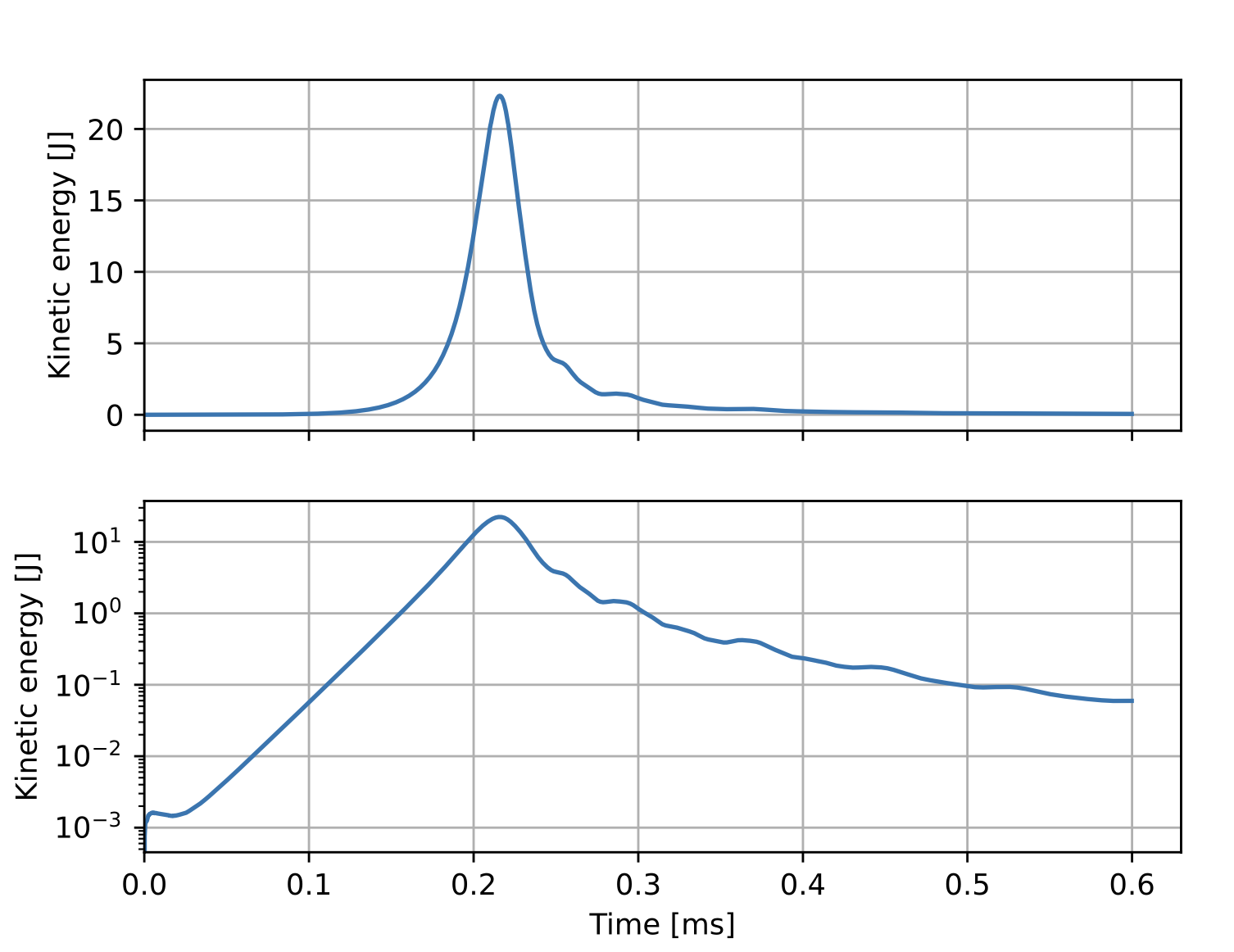
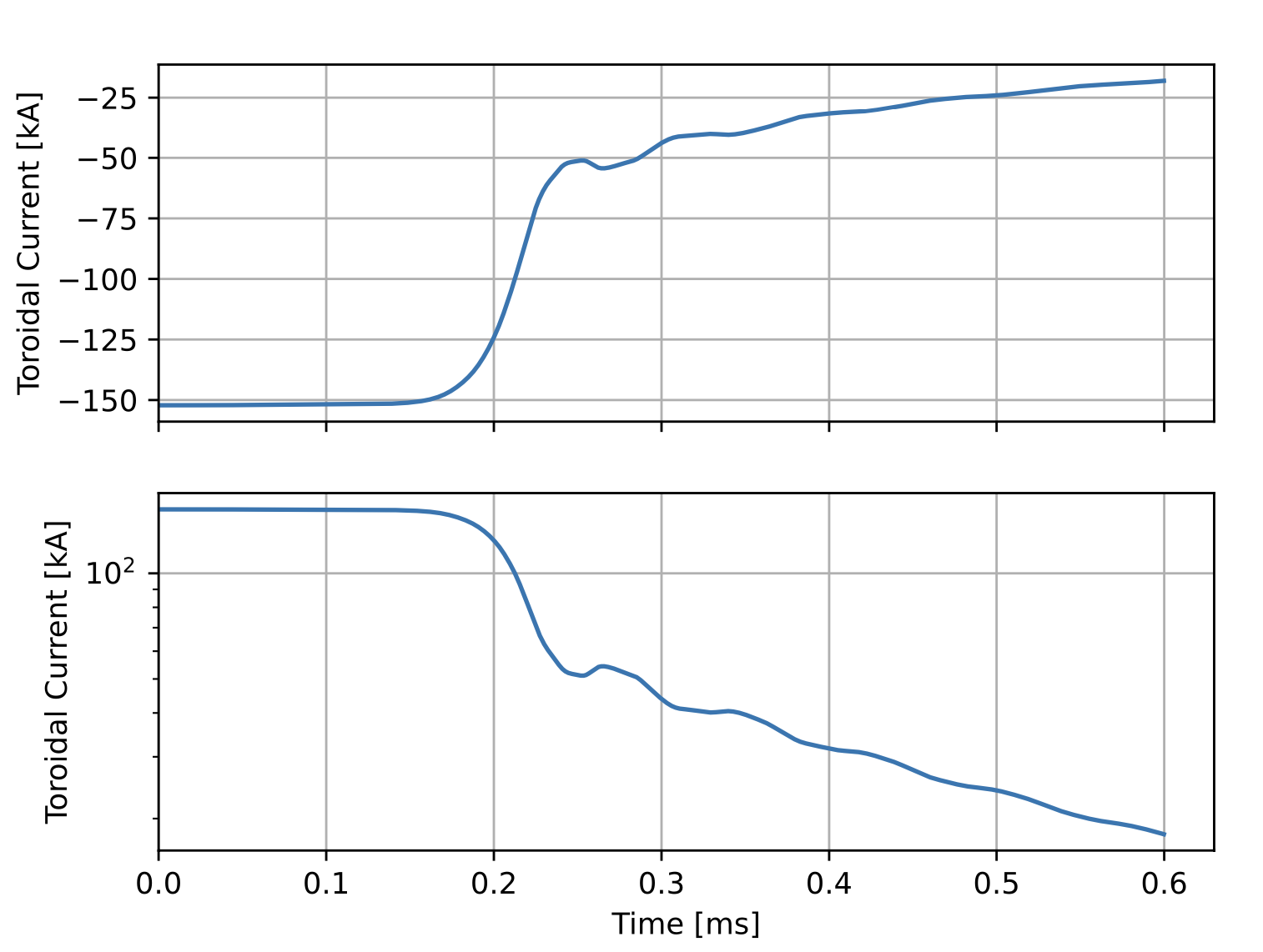
Several quantities are also recorded to a history file xmhd.hist during the simulation, including the toroidal current (where the symmetry axis is specified by xmhd_taxis). The data in the history file may be plotted using the script plot_mug_hist.py, which is located in src/utilities/scripts or python directories for the repository and an installation respectively.
- Note
- OFT plotting scripts require the python packages
numpyandmatplotlibas well as path access to the python modules provided inpythonfor installations orsrc/utilitiesin the repo.
Input file
Below is an input file which can be used with this example in a parallel environment. This example should not be run with only a single process as solving the time-depedent MHD equations is significantly more challenging than previous examples. For more information on the options in the xmhd_options group see xmhd_run.
&runtime_options
 ppn=1
 debug=0
/

&mesh_options
 meshname='test'
 cad_type=0
 nlevels=2
 nbase=1
 grid_order=2
 fix_boundary=T
/

&native_mesh_options
 filename='cyl_tilt.h5'
/

&sph_tilt_options
 order=2
 linear=F
 b0_scale=1.e-1
 b1_scale=1.e-4
 n0=1.E19
 t0=3.
 plot_run=F
 pm=F
/

&xmhd_options
 xmhd_adv_den=F    ! Do not advance density
 xmhd_adv_temp=F   ! Do not advance temperature
 bbc='bc'          ! Perfectly-conducting BC for B-field
 vbc='all'         ! Zero-flow BC for velocity
 dt=2.e-7          ! Maximum time step
 eta=1.            ! Resistivity
 nu_par=10.        ! Fluid viscosity
 nsteps=3000       ! Number of time steps to take
 rst_freq=10       ! Restart file frequency
 lin_tol=1.E-10    ! Linear solver tolerance
 nl_tol=1.E-5      ! Non-linear solver tolerance
 xmhd_mfnk=T       ! Use matrix-free Jacobian operator
 rst_ind=0         ! Index of file to restart from (0 -> use subroutine arguments)
 ittarget=40       ! Target for # of linear iterations per time step
 mu_ion=2.         ! Ion mass (atomic units)
 xmhd_prefreq=20   ! Preconditioner update frequency
/
Solver specification
Time dependent MHD solvers are accelerated significantly by the use of a more sophisticated preconditioner than the default method. Below is an example oft_in.xml file that constructs an appropriate ILU(0) preconditioner. Currently, this preconditioner method is the suggested starting preconditioner for all time-dependent MHD solves.
This solver can be used by specifying both the FORTRAN input and XML input files to the executable as below.
~$ ./MUG_sph_tilt oft.in oft_in.xml
Post-Processing options
During the simulation the evolution of some global quantities is written to the history file xmhd.hist. A utility script (plot_mug_hist.py located in bin after installation) is included as part of OFT for plotting the signals in this file. This is useful for monitoring general progress of the simulation as well as numerical parameters like the iteration count and solver time. Using this script we can see the instability growth and relaxation of the initial magnetic equilibrium to the lowest energy state.
~$ python plot_mug_hist.py xmhd.hist
Creating plot files
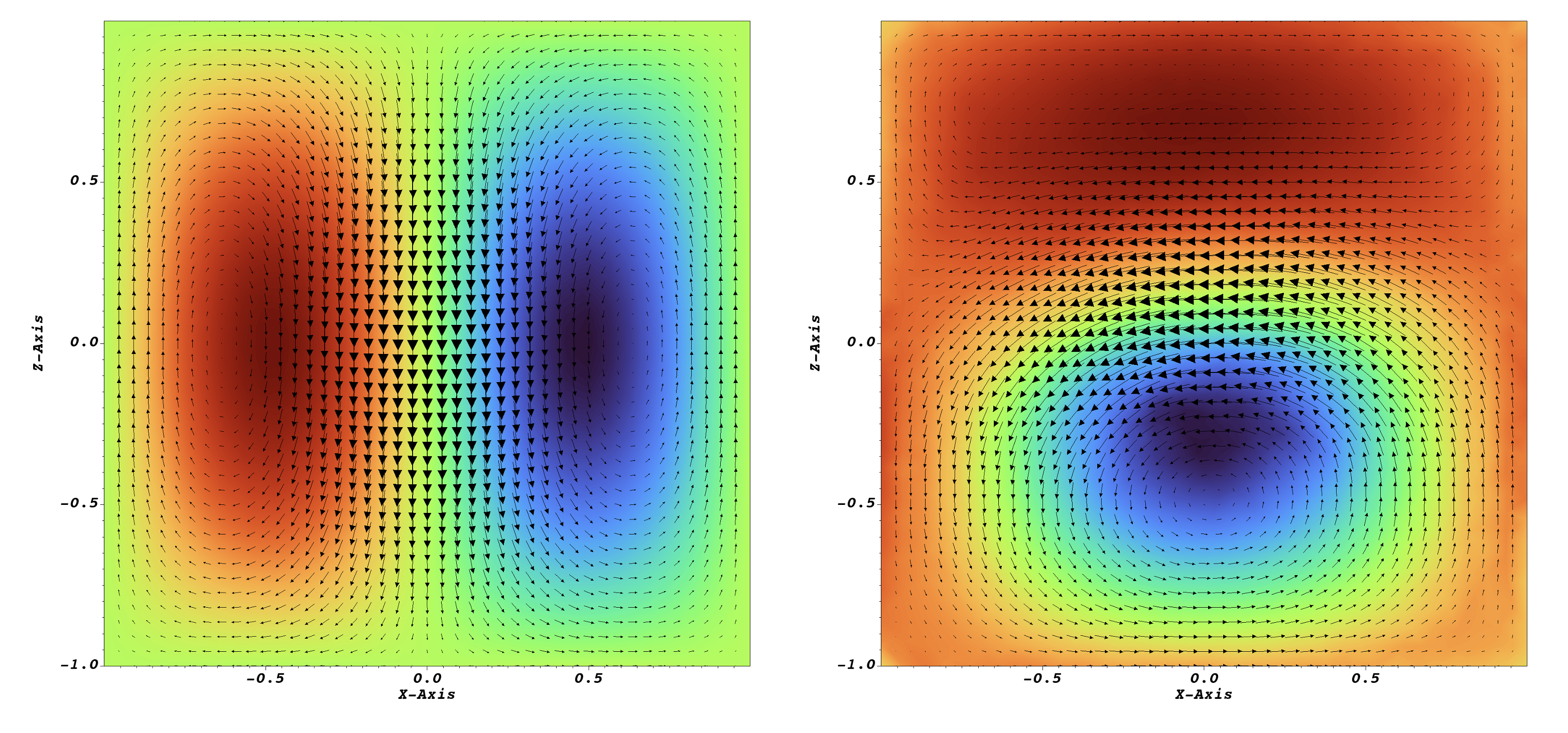
To generate 3D plots, and perform additional diagnostic sampling (see oft_xmhd_probe), a plot run can be performed by setting plot_run=T in the sph_tilt_options input group, which calls xmhd_plot. With this option additional run time options are available in the xmhd_plot_options group that control how restart files are sampled for plotting.
&xmhd_plot_options
 t0=1.E-8
 dt=1.E-5
 rst_start=0
 rst_end=3000
/
Once the post-processing run is complete bin/build_xdmf.py can be used to generate *.xmf files that can be loaded by VisIt, ParaView, or other visualization programs.
Mesh Creation
A mesh file cyl_tilt.h5 is provided with this example. Instructions to generate your own mesh for the geometry using CUBIT and GMSH.
Meshing with CUBIT
A suitable mesh for this example, with radius of 1m and height of 2m, can be created using the CUBIT script below.
reset

create Cylinder height 2 radius 1

volume 1 scheme Tetmesh
set tetmesher interior points on
set tetmesher optimize level 3 optimize overconstrained  off sliver  off
set tetmesher boundary recovery  off
volume 1 size .2
mesh volume 1

set duplicate block elements off
block 1 add volume 1
block 1 element type tetra10

set large exodus file on
export Genesis  "cyl_tilt.g" overwrite block 1
Once complete the mesh should be converted into the native mesh format using the convert_cubit.py script as below. The script is located in bin following installation or src/utilities in the base repo.
~$ python convert_cubit.py --in_file=cyl_tilt.g
Meshing with Gmsh
If the CUBIT mesh generation codes is not avilable the mesh can be created using the Gmsh code and the geometry script below.
Coherence;
Point(1) = {0, 0, 0, 1.0};
Point(2) = {1, 0, 0, 1.0};
Point(3) = {0, 1, 0, 1.0};
Point(4) = {-1, 0, 0, 1.0};
Point(5) = {0, -1, 0, 1.0};
Circle(1) = {2, 1, 3};
Circle(2) = {3, 1, 4};
Circle(3) = {4, 1, 5};
Circle(4) = {5, 1, 2};
Line Loop(5) = {2, 3, 4, 1};
Plane Surface(6) = {5};
Extrude {0, 0, 2} {
  Surface{6};
}
To generate a mesh, with resolution matching the Cubit example above, place the script contents in a file called cyl_tilt.geo and run the following command.
~$ gmsh -3 -format mesh -optimize -clscale .2 -order 2 -o cyl_tilt.mesh cyl_tilt.geo
Once complete the mesh should be converted into the native mesh format using the convert_gmsh.py script as below. The script is located in bin following installation or src/utilities in the base repo.
~$ python convert_gmsh.py --in_file=cyl_tilt.mesh