In this example we demonstrate how to run a time-domain simulation for a simple ThinCurr model of a cylinder.

Note: Running this example requires the h5py and pyvista python packages, which are installable using pip or other standard methods.

import struct
import sys
import os
import h5py
import numpy as np
import matplotlib.pyplot as plt
import matplotlib.lines as mlines
import pyvista
pyvista.set_jupyter_backend('static') # Comment to enable interactive PyVista plots
plt.rcParams['figure.figsize']=(6,6)
plt.rcParams['font.weight']='bold'
plt.rcParams['axes.labelweight']='bold'
plt.rcParams['lines.linewidth']=2
plt.rcParams['lines.markeredgewidth']=2
%matplotlib inline
%config InlineBackend.figure_format = "retina"

Load ThinCurr library

To load the ThinCurr python module we need to tell python where to the module is located. This can be done either through the PYTHONPATH environment variable or within a script using sys.path.append() as below, where we look for the environement variable OFT_ROOTPATH to provide the path to where the OpenFUSIONToolkit is installed (/Applications/OFT for binaries on macOS).

thincurr_python_path = os.getenv('OFT_ROOTPATH')
if thincurr_python_path is not None:
    sys.path.append(os.path.join(thincurr_python_path,'python'))
from OpenFUSIONToolkit.ThinCurr import ThinCurr
from OpenFUSIONToolkit.ThinCurr.sensor import circular_flux_loop, save_sensors
from OpenFUSIONToolkit.util import build_XDMF, mu0
from OpenFUSIONToolkit.io import histfile

Setup ThinCurr model

We now create a ThinCurr instance to use for equilibrium calculations. As this is a larger model, we use nthreads=4 to increase the number of cores used for the calculation. Once created, we setup the model from an existing HDF5 and XML mesh definition using setup_model(). We also initialize I/O for this model using setup_io() to enable output of plotting files for 3D visualization in VisIt, Paraview, or using pyvista below.

tw_torus = ThinCurr(nthreads=4)
tw_torus.setup_model(mesh_file='thincurr_ex-cyl.h5',xml_filename='oft_in.xml')
tw_torus.setup_io()

#----------------------------------------------
Open FUSION Toolkit Initialized
Development branch:   main
Revision id:          8440e61
Parallelization Info:
  Not compiled with MPI
  # of OpenMP threads =    4
Fortran input file    = oftpyin                                                                         
XML input file        = none                                                                            
Integer Precisions    =    4   8
Float Precisions      =    4   8  16
Complex Precisions    =    4   8
LA backend            = native
#----------------------------------------------


Creating thin-wall model
 Orientation depth =         895
  Loading V(t) driver coils
  Loading I(t) driver coils

  # of points    =          795
  # of edges     =         2259
  # of cells     =         1464
  # of holes     =            1
  # of Vcoils    =            0
  # of closures  =            0
  # of Icoils    =            1

  Building holes

  Loading region resistivity:
     1  1.2570E-05

Define flux loop sensors

To visualize the results we define two circular flux loops at R=0.9 m, just inside the cylinder. While every sensor in ThinCurr is a flux loop, helper classes for defining specific types of common sensors (eg. circular loop or Mirnovs) are available in OpenFUSIONToolkit.ThinCurr.sensor, which also contains the save_sensors() function for saving this information to a ThinCurr-compatible file format.

sensors = [
    circular_flux_loop(0.25,0.9,'Floop_1'),
    circular_flux_loop(0.5,0.9,'Floop_2')
]
save_sensors(sensors)
Msensor, Msc, sensor_obj = tw_torus.compute_Msensor('floops.loc')

 Loading floop information:
   # of floops =           2
 Building element->sensor inductance matrix
 Building coil->sensor inductance matrix

Compute self-inductance and resistivity matrices

With the model setup, we can now compute the self-inductance and resistivity matrices. A numpy version of the self-inductance matrix will be stored at tw_plate.Lmat. By default the resistivity matrix is not moved to python as it is sparse and converting to dense representation would require an increase in memory. These matrices correspond to the \(\textrm{L}\) and \(\textrm{R}\) matrices for the physical system

\(\textrm{L} \frac{\partial I}{\partial t} + \textrm{R} I = V\)

Note: For larger models calculating the self-inductance may take some time due to the \(N^2\) interaction of the elements (see ThinCurr Python Example: Using HODLR approximation for more information).

Mc = tw_torus.compute_Mcoil()
tw_torus.compute_Lmat()
tw_torus.compute_Rmat()

 Building coil<->element inductance matrices
     Time =  0s          
 Building coil<->coil inductance matrix
 Building element<->element self inductance matrix
     Time =  0s          
 Building resistivity matrix

Run time-domain simulation

With the model fully defined we can now use run_td() to perform a time-domain simulation. In this case we simulate 80 ms using a timestep of 0.2 ms (400 steps). We also specify using a direct solver for the time-advance (direct=True) and set the current in the single I-coil defined in the XML input file as a function of time (coil_currs), where the first column specifies time points in ascending order and the remaining columns specify coil currents at each time point.

dt = 2.E-4
nsteps = 400
coil_currs = np.array([
    [0.0, 0.0],
    [2.E-2, 1.E3],
    [1.0, 1.E3]
])
tw_torus.run_td(dt,nsteps,status_freq=10,coil_currs=coil_currs,sensor_obj=sensor_obj,direct=True)

 Starting simulation
 Starting factorization
 Inverting real matrix
   Time =    8.0610000000000005E-003
 Timestep           10   2.00000009E-03   1.49562431E-03           1
 Timestep           20   4.00000019E-03   2.79602758E-03           1
 Timestep           30   6.00000005E-03   3.89465201E-03           1
 Timestep           40   8.00000038E-03   4.82152030E-03           1
 Timestep           50   9.99999978E-03   5.60256746E-03           1
 Timestep           60   1.20000001E-02   6.26014080E-03           1
 Timestep           70   1.40000004E-02   6.81338552E-03           1
 Timestep           80   1.60000008E-02   7.27861980E-03           1
 Timestep           90   1.79999992E-02   7.66969658E-03           1
 Timestep          100   1.99999996E-02   7.95726292E-03           1
 Timestep          110   2.19999999E-02   6.74793730E-03           1
 Timestep          120   2.40000002E-02   5.68624772E-03           1
 Timestep          130   2.60000005E-02   4.78724064E-03           1
 Timestep          140   2.80000009E-02   4.02757991E-03           1
 Timestep          150   2.99999993E-02   3.38672171E-03           1
 Timestep          160   3.20000015E-02   2.84674857E-03           1
 Timestep          170   3.40000018E-02   2.39218818E-03           1
 Timestep          180   3.59999985E-02   2.00978271E-03           1
 Timestep          190   3.79999988E-02   1.68823614E-03           1
 Timestep          200   3.99999991E-02   1.41796179E-03           1
 Timestep          210   4.19999994E-02   1.19084632E-03           1
 Timestep          220   4.39999998E-02   1.00003765E-03           1
 Timestep          230   4.60000001E-02   8.39756802E-04           1
 Timestep          240   4.80000004E-02   7.05135928E-04           1
 Timestep          250   5.00000007E-02   5.92077384E-04           1
 Timestep          260   5.20000011E-02   4.97134111E-04           1
 Timestep          270   5.40000014E-02   4.17407835E-04           1
 Timestep          280   5.60000017E-02   3.50462447E-04           1
 Timestep          290   5.79999983E-02   2.94250814E-04           1
 Timestep          300   5.99999987E-02   2.47053104E-04           1
 Timestep          310   6.19999990E-02   2.07424571E-04           1
 Timestep          320   6.40000030E-02   1.74151835E-04           1
 Timestep          330   6.59999996E-02   1.46215840E-04           1
 Timestep          340   6.80000037E-02   1.22760786E-04           1
 Timestep          350   7.00000003E-02   1.03068058E-04           1
 Timestep          360   7.19999969E-02   8.65342372E-05           1
 Timestep          370   7.40000010E-02   7.26526559E-05           1
 Timestep          380   7.59999976E-02   6.09978961E-05           1
 Timestep          390   7.80000016E-02   5.12127554E-05           1
 Timestep          400   7.99999982E-02   4.29973261E-05           1

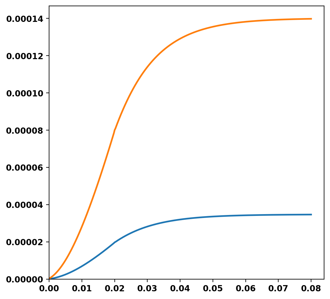
Plot sensor signals

We can now plot the signals from the two flux loops defined above as a function of time. During the time-domain run this information is stored in OFT's binary history file format, which can be read using the histfile class. This class stores the resulting signals in a Python dict-like representation.

hist_file = histfile('floops.hist')
print(hist_file)
 
fig, ax = plt.subplots(1,1)
ax.plot(hist_file['time'],hist_file['Floop_1'])
ax.plot(hist_file['time'],hist_file['Floop_2'])
ax.set_ylim(bottom=0.0)
_ = ax.set_xlim(left=0.0)

OFT History file: floops.hist
  Number of fields = 3
  Number of entries = 401

  Fields:
    time: Simulation time [s] (d1)
    Floop_1: No description (d1)
    Floop_2: No description (d1)

Generate plot files

After completing the simulation we can generate plot files using tw_torus.plot_td(). Plot files are saved at a fixed timestep interval, specified by the nplot argument to run_td() with a default value of 10.

Once all fields have been saved for plotting tw_torus.build_XDMF() to generate the XDMF descriptor files for plotting with VisIt of Paraview.

tw_torus.plot_td(nsteps,sensor_obj=sensor_obj)

tw_torus.build_XDMF()

 Post-processing simulation
Removing old Xdmf files
Creating output files

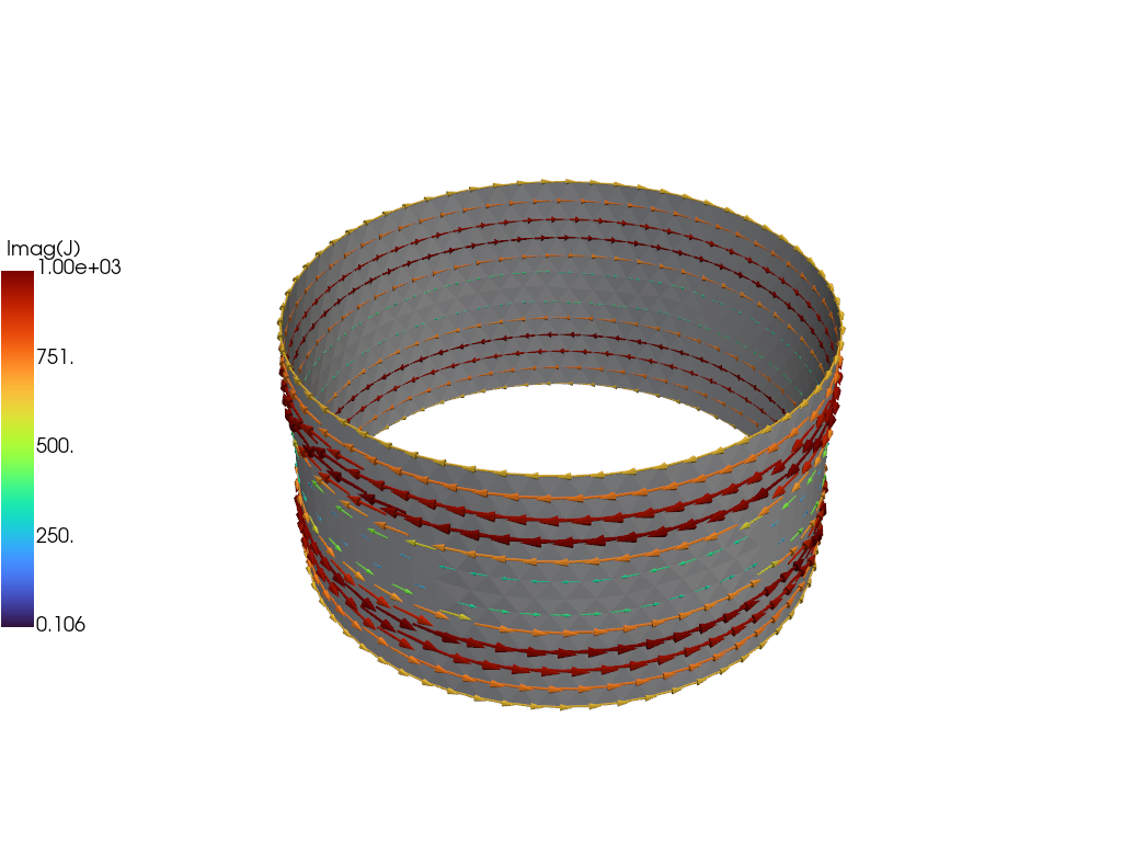
Plot current fields using pyvista

For demonstration purposes we now plot the the solution at the end of the driven phase using pyvista. For more information on the steps in this block see ThinCurr Python Example: Compute eigenstates in a plate

# Load mesh and current from plot files
with h5py.File('mesh.0001.h5','r') as h5_file:
    r = np.asarray(h5_file['R_surf'])
    lc = np.asarray(h5_file['LC_surf'])
with h5py.File('vector_dump.0001.h5','r') as h5_file:
    J = np.asarray(h5_file['J_v0011'])
 
# Create pyvista mesh for plotting
celltypes = np.array([pyvista.CellType.TRIANGLE for _ in range(lc.shape[0])], dtype=np.int8)
cells = np.insert(lc, [0,], 3, axis=1)
grid = pyvista.UnstructuredGrid(cells, celltypes, r)
 
# Plot mesh and current density using PyVista
p = pyvista.Plotter()
grid["vectors"] = J
grid.set_active_vectors("vectors")
scale = 0.2/(np.linalg.norm(J,axis=1)).max()
arrows = grid.glyph(scale="vectors", orient="vectors", factor=scale)
p.add_mesh(arrows, cmap="turbo", scalar_bar_args={'title': "Imag(J)", "vertical": True, "position_y":0.25, "position_x": 0.0})
p.add_mesh(grid, color="white", opacity=1.0, show_edges=False)
p.show()