In this example we demonstrate how to compute eigenvalues/eigenvectors and run a time-domain simulation for a large ThinCurr model using HODLR matrix compression.
- Note
- Running this example requires the h5py and pyvista python packages, which are installable using
pipor other standard methods.
Load ThinCurr library
To load the ThinCurr python module we need to tell python where to the module is located. This can be done either through the PYTHONPATH environment variable or within a script using sys.path.append() as below, where we look for the environement variable OFT_ROOTPATH to provide the path to where the OpenFUSIONToolkit is installed (/Applications/OFT for binaries on macOS).
Compute eigenvalues
Setup ThinCurr model
We now create a ThinCurr instance to use for equilibrium calculations. As this is a larger model, we use nthreads=4 to increase the number of cores used for the calculation. Once created, we setup the model from an existing HDF5 and XML mesh definition using setup_model(). We also initialize I/O for this model using setup_io() to enable output of plotting files for 3D visualization in VisIt, Paraview, or using pyvista below.
#----------------------------------------------
Open FUSION Toolkit Initialized
Development branch:   main
Revision id:          8440e61
Parallelization Info:
  Not compiled with MPI
  # of OpenMP threads =    4
Fortran input file    = oftpyin
XML input file        = none
Integer Precisions    =    4   8
Float Precisions      =    4   8  16
Complex Precisions    =    4   8
LA backend            = native
#----------------------------------------------


Creating thin-wall model
 Orientation depth =       26500
  Loading V(t) driver coils
  Loading I(t) driver coils

  # of points    =        22580
  # of edges     =        67150
  # of cells     =        44560
  # of holes     =           11
  # of Vcoils    =            0
  # of closures  =            0
  # of Icoils    =            1

  Building holes

  Loading region resistivity:
     1  1.2570E-05
 Loading floop information:
   # of floops =           3
 Building element->sensor inductance matrix
 Building coil->sensor inductance matrix
Compute inductance and resistivity matrices
With the model setup, we can now compute the self-inductance matrix using HODLR. When HODLR is used the result is a pointer to the Fortran operator, which is stored at tw_torus.Lmat_hodlr. As in any other case, by default, the resistivity matrix is not moved to python as it is sparse and converting to dense representation would require an increase in memory. These matrices correspond to the \(\textrm{L}\) and \(\textrm{R}\) matrices for the physical system
\(\textrm{L} \frac{\partial I}{\partial t} + \textrm{R} I = V\)
- Note
- Even though HODLR should significantly accelerate the construction of the self-inductance matrix (see ThinCurr Example: Using HODLR approximation for more information) this process may still take some time to complete.
- The non-zero savings achieved by HODLR compression is reported after the operator is built. Where in this case only 6% of the original memory is needed resulting in a reduction from > 3 GB to ~ 230 MB (over 10x smaller)!
 Building coil<->element inductance matrices
     Time =  0s
 Building coil<->coil inductance matrix
 Partitioning grid for block low rank compressed operators
   nBlocks =                  32
   Avg block size =          686
   # of SVD =                167
   # of ACA =                161

 Building block low rank inductance operator
   Building hole and Vcoil columns
   Building diagonal blocks
     10%
     20%
     30%
     40%
     50%
     60%
     70%
     80%
     90%
   Building off-diagonal blocks using ACA+
     10%
     20%
     30%
     40%
     50%
     60%
     70%
     80%
     90%
     Compression ratio:   6.1%  ( 2.94E+07/ 4.82E+08)
     Time =  1m 49s
   Saving HODLR matrix to file: HOLDR_L.save
Building resistivity matrix
Compute eigenvalues/eigenvectors for the plate model
With \(\textrm{L}\) and \(\textrm{R}\) matrices we can now compute the eigenvalues and eigenvectors of the system \(\textrm{L} I = \lambda \textrm{R} I\), where the eigenvalues \(\lambda = \tau_{L/R}\) are the decay time-constants of the current distribution corresponding to each eigenvector.
 Starting eigenvalue solve
   Time =    3.1256420000000000
 Eigenvalues
      3.8803529724910198E-002
      2.3122422873188293E-002
      2.3121316748127611E-002
      2.1444722232381232E-002
      2.0605571170591544E-002
Save data for plotting
The resulting currents can be saved for plotting using tw_torus.save_current(). Here we save each of the five eigenvectors for visualization. Once all fields have been saved for plotting tw_torus.build_XDMF() to generate the XDMF descriptor files for plotting with VisIt of Paraview.
Removing old Xdmf files
Creating output files
Plot current fields using pyvista
For demonstration purposes we now plot the first eigenvector using pyvista.
Load data from plot files
To plot the fields we must load in the mesh from the plot files.
- Note
- In the future this will be handled by dedicated python functions, but we show it here at the moment for demonstration purposes.
Create pyvista mesh for plotting
Now we create a pyvista/VTK mesh from the loaded information and add the vector field to the mesh.
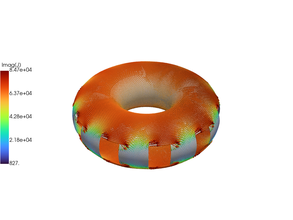
Generate vector plot
Finally we plot the current vectors on the plate showing the longest-lived eddy current structure, which corresponds to a large circulation on the plate.
Run time-domain simulation
 Starting simulation
 Timestep           10   2.00000009E-03   22.7324562              32
 Timestep           20   4.00000019E-03   44.1192436              18
 Timestep           30   6.00000005E-03   42.2026978              32
 Timestep           40   8.00000038E-03   39.9049377              32
 Timestep           50   9.99999978E-03   37.7692719              32
 Timestep           60   1.20000001E-02   35.7698593              32
 Timestep           70   1.40000004E-02   33.8907852              32
 Timestep           80   1.60000008E-02   32.1206093              32
 Timestep           90   1.79999992E-02   30.4503784              32
 Timestep          100   1.99999996E-02   28.8726749              32
 Timestep          110   2.19999999E-02   27.3811474              32
 Timestep          120   2.40000002E-02   25.9701881              32
 Timestep          130   2.60000005E-02   24.6347980              32
 Timestep          140   2.80000009E-02   23.3704281              32
 Timestep          150   2.99999993E-02   22.1729164              32
 Timestep          160   3.20000015E-02   21.0384293              32
 Timestep          170   3.40000018E-02   19.9634113              32
 Timestep          180   3.59999985E-02   18.9445419              32
 Timestep          190   3.79999988E-02   17.9787292              32
 Timestep          200   3.99999991E-02   17.0630741              32
Generate plot files from run
 Building block low rank magnetic field operator
   Building hole and Vcoil columns
   Building diagonal blocks
     10%
     20%
     30%
     40%
     50%
     60%
     70%
     80%
     90%
   Building off-diagonal blocks using ACA+
     10%
     20%
     30%
     40%
     50%
     60%
     70%
     80%
     90%
     Compression ratio:   7.1%  ( 1.06E+08/ 1.49E+09)
     Time =  3m 35s
   Saving HODLR matrix from file: HODLR_B.save
 Post-processing simulation
Removing old Xdmf files
Creating output files
Load sensor signals from time-domain run
OFT History file: floops.hist
  Number of fields = 4
  Number of entries = 201

  Fields:
    time: Simulation time [s] (d1)
    Bz_1: No description (d1)
    Bz_2: No description (d1)
    Bz_3: No description (d1)