In this example we demonstrate how to compute eigenvalues and eigenvectors for a simple ThinCurr model.
- Note
- Running this example requires the h5py and pyvista python packages, which are installable using
pipor other standard methods.
Load ThinCurr library
To load the ThinCurr python module we need to tell python where to the module is located. This can be done either through the PYTHONPATH environment variable or within a script using sys.path.append() as below, where we look for the environement variable OFT_ROOTPATH to provide the path to where the OpenFUSIONToolkit is installed (/Applications/OFT for binaries on macOS).
Compute eigenvalues
Setup ThinCurr model
We now create a ThinCurr instance to use for equilibrium calculations. Once created, we setup the model from an existing HDF5 and XML mesh definition using setup_model(). We also initialize I/O for this model using setup_io() to enable output of plotting files for 3D visualization in VisIt, Paraview, or using pyvista below.
#----------------------------------------------
Open FUSION Toolkit Initialized
Development branch:   main
Revision id:          8440e61
Parallelization Info:
  Not compiled with MPI
  # of OpenMP threads =    2
Fortran input file    = oftpyin
XML input file        = none
Integer Precisions    =    4   8
Float Precisions      =    4   8  16
Complex Precisions    =    4   8
LA backend            = native
#----------------------------------------------


Creating thin-wall model
 Orientation depth =         747
  Loading V(t) driver coils
  Loading I(t) driver coils

  # of points    =          492
  # of edges     =         1393
  # of cells     =          902
  # of holes     =            0
  # of Vcoils    =            0
  # of closures  =            0
  # of Icoils    =            1

  Building holes

  Loading region resistivity:
     1  1.2570E-05
Compute self-inductance and resistivity matrices
With the model setup, we can now compute the self-inductance and resistivity matrices. A numpy version of the self-inductance matrix will be stored at tw_plate.Lmat. By default the resistivity matrix is not moved to python as it is sparse and converting to dense representation would require an increase in memory. These matrices correspond to the \(\textrm{L}\) and \(\textrm{R}\) matrices for the physical system
\(\textrm{L} \frac{\partial I}{\partial t} + \textrm{R} I = V\)
- Note
- For larger models calculating the self-inductance may take some time due to the \(N^2\) interaction of the elements (see ThinCurr Python Example: Using HODLR approximation for more information).
 Building element<->element self inductance matrix
     Time =  0s
 Building resistivity matrix
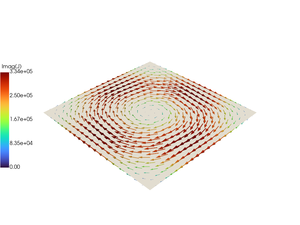
Compute eigenvalues/eigenvectors for the plate model
With \(\textrm{L}\) and \(\textrm{R}\) matrices we can now compute the eigenvalues and eigenvectors of the system \(\textrm{L} I = \lambda \textrm{R} I\), where the eigenvalues \(\lambda = \tau_{L/R}\) are the decay time-constants of the current distribution corresponding to each eigenvector.
 Starting eigenvalue solve
   Time =    3.5599999999999998E-003
 Eigenvalues
      9.7328555499775465E-003
      6.5304273569129073E-003
      6.5303149629831981E-003
      5.2500818095550413E-003
      4.7031013858612070E-003
Save data for plotting
The resulting currents can be saved for plotting using tw_plate.save_current(). Here we save each of the five eigenvectors for visualization. Once all fields have been saved for plotting tw_plate.build_XDMF() to generate the XDMF descriptor files for plotting with VisIt of Paraview.
Removing old Xdmf files
Creating output files
Plot current fields using pyvista
For demonstration purposes we now plot the first eigenvector using pyvista.
Load data from plot files
To plot the fields we must load in the mesh from the plot files.
- Note
- In the future this will be handled by dedicated python functions, but we show it here at the moment for demonstration purposes.
Create pyvista mesh for plotting
Now we create a pyvista/VTK mesh from the loaded information and add the vector field to the mesh.
Plot current vectors on surface
Finally we plot the current vectors on the plate showing the longest-lived eddy current structure, which corresponds to a large circulation on the plate.