 |
The Open FUSION Toolkit 26.9
An open-source framework for fusion and plasma science and engineering
|
Loading...
Searching...
No Matches
|
The Open FUSION Toolkit 26.9
An open-source framework for fusion and plasma science and engineering
|
This is based on the open source SPARC data published by Commonwealth Fusion Systems (CFS) in the SPARCPublic repository. We reconstruct the Primary Reference Discharge (PRD), the SPARC baseline H-mode scenario ( \(R_0 = 1.85\) m, \(B_0 = 12.2\) T, \(I_p = 8.7\) MA), described in Creely et al, "Overview of the SPARC tokamak", J. Plasma Phys. 86(5), 865860502 (2020). https://doi.org/10.1017/S0022377820001257
All files are openly available on GitHub at: https://github.com/cfs-energy/SPARCPublic/
This notebook uses the mesh built in TokaMaker Meshing Example: Building a mesh for SPARC (SPARC_public_make_mesh.ipynb) and takes its equilibrium parameters and profiles from the double-null FreeGS gEQDSK, 2 - SPARC_DN_PRD_freegs_20221013, in the PrimaryReferenceDischarge folder of the public SPARC repo. The gEQDSK is read directly from the repository.
To load the TokaMaker python module we need to tell python where to the module is located. This can be done either through the PYTHONPATH environment variable or using within a script using sys.path.append() as below, where we look for the environement variable OFT_ROOTPATH to provide the path to where the OpenFUSIONToolkit is installed (/Applications/OFT on macOS).
A dictionary containing the equilibrium information is obtained using read_eqdsk(). The dictionary contains multiple key quantities useful for reproducing the equilibrium in TokaMaker:
The SPARC gEQDSK is read straight from SPARCPublic. read_eqdsk() takes a path rather than a file object, so we stage the download in a temporary file and delete it immediately afterwards.
Fetching 2 - SPARC_DN_PRD_freegs_20221013 from SPARCPublic... done.
  Ip      = 8.70 MA
  F0      = 22.49 T.m  (B0 = 12.16 T at R0 = 1.85 m)
  p_axis  = 2.60 MPa
  axis    = (1.890, -0.000) m
We now create a OFT_env instance for execution using two threads and a TokaMaker instance to use for equilibrium calculations. Note at present only a single TokaMaker instance can be used per python kernel, so this command should only be called once in a given Jupyter notebook or python script. In the future this restriction may be relaxed.
#----------------------------------------------
Open FUSION Toolkit Initialized
Development branch:    tmtx_updates_1
Revision id:           22e8b4e
Parallelization Info:
  Not compiled with MPI
  # of OpenMP threads =    2
Integer Precisions    =    4   8
Float Precisions      =    4   8  16
Complex Precisions    =    4   8
LA backend            = native
#----------------------------------------------
Sometimes it is useful to modify the default TokaMaker settings. Here we update one setting to help with convergence:
Settings can be modified before running setup() or at any time during execution by adjusting desired values and then calling update_settings().
Now we load the mesh generated in TokaMaker Meshing Example: Building a mesh for SPARC using load_gs_mesh() and setup_mesh. Then we use setup_regions(), passing the conductor and coil dictionaries for the mesh, to define the different region types. Finally, we call setup() to setup the required solver objects. During this call we can specify the desired element order (min=2, max=4) and the toroidal field through F0 = B0*R0, where B0 is the toroidal field at a reference location R0.
**** Loading OFT surface mesh

**** Generating surface grid level  1
  Generating boundary domain linkage
  Mesh statistics:
    Area         =  2.900E+01
    # of points  =   18989
    # of edges   =   56604
    # of cells   =   37616
    # of boundary points =     360
    # of boundary edges  =     360
    # of boundary cells  =     360
  Resolution statistics:
    hmin =  1.000E-03
    hrms =  4.468E-02
    hmax =  9.258E-02
  Surface grounded at vertex    3175


**** Creating Lagrange FE space
  Order  =    2
  Minlev =   -1

 Computing flux BC matrix
 Inverting real matrix
   Time =    1.5264000000000000E-002
Like many elongated equilibria, the equilibrium we seek to compute below is vertically unstable ( \(\kappa \approx 1.95\)). Where the ARC example repurposed its outermost PF pair for this, SPARC has a dedicated pair of in-vessel vertical stability coils, VS1U and VS1L, which we drive anti-symmetrically using the set_coil_vsc() method. This matches the device description itself, where VS1L carries turns_with_sign = -1 on every turn — i.e. the pair is wound in opposition.
For the inverse case we define a target for the plasma current and the peak plasma pressure, which occurs on the magnetic axis. Both are taken from the gEQDSK.
In order to constrain the shape of the plasma we can utilize two types of constraints:
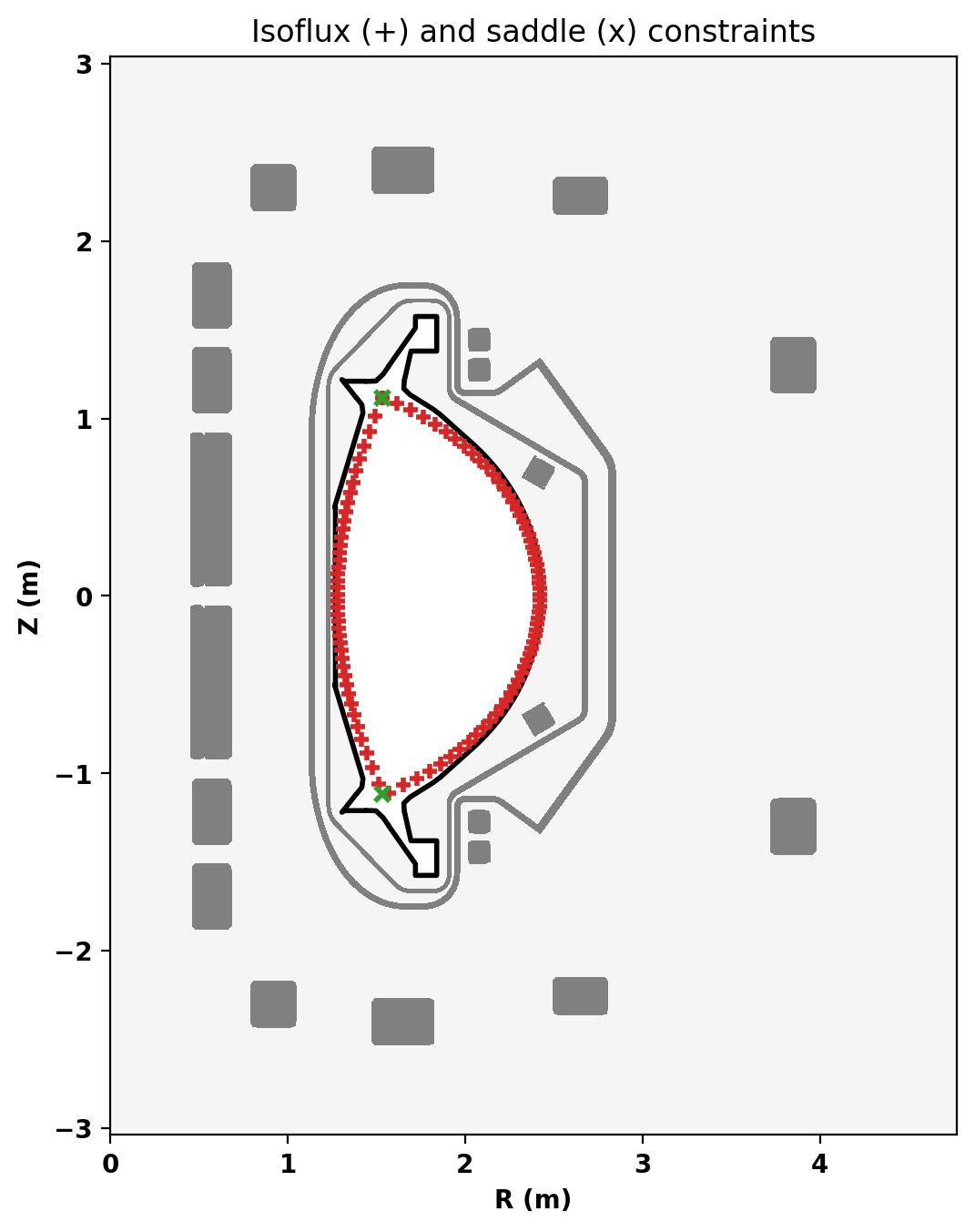
Here we use the contour defining the last closed flux surface as our isoflux constraint. Unlike the ARC example we also set saddle targets: this is a double-null discharge, and with isoflux constraints alone the solver settles into a limited topology rather than a diverted one.
We need both X-points, and because the PRD is an up-down symmetric double null they must be exact mirrors of each other. We take the upper X-point from the boundary extremum and mirror it in \(Z\) to obtain the lower one.
Upper X-point: R = 1.5312 m, Z = +1.1168 m
Lower X-point: R = 1.5312 m, Z = -1.1168 m
Before solving it is worth looking at what we have actually asked the solver for. Below we overlay the constraints on the machine geometry using plot_constraints(): the isoflux points (red +, the gEQDSK boundary contour) and the saddle points (green x, the two X-points). Both X-points should sit inside the divertor region of the limiter, and the isoflux contour should lie comfortably inside the vessel.
Although TokaMaker has a "default" profile for the F*F' and P' terms this should almost never be used and one should instead choose an appropriate flux function for their application. In this case we use the P' and F*F' profiles directly from the gEQDSK we are working to reproduce.
We can now compute a free-boundary equilibrium using these constraints. Note that before running a calculation for the first time we must initialize the flux function \(\psi\), which can be done using init_psi(). This subroutine initializes the flux using the specified Ip_target from above, which is evenly distributed over the entire plasma region or only with a boundary defined using a center point (R,Z), minor radius (a), and elongation and triangularity. Coil currents are also initialized at this point using the constraints above and this uniform plasma current initialization.
Rather than hard-coding the initialization shape we measure it from the gEQDSK boundary contour, which gives \(a = 0.57\) m, \(\kappa = 1.96\) and \(\delta = 0.56\) for the PRD.
solve() is then called to compute a self-consitent Grad-Shafranov equilibrium. If the result variable (err_flag) is zero then the solution has converged to the desired tolerance ( \(10^{-6}\) by default).
Starting non-linear GS solver
     1  7.2949E-01  2.4769E-06  1.8559E-01  1.9085E+00  1.1440E-03  7.4755E+02
     2  1.6150E+00  1.5030E-06  7.3857E-02  1.9005E+00  1.2507E-03  5.8926E+02
     3  1.8070E+00  1.3443E-06  3.0918E-02  1.8960E+00  1.2681E-03  4.8239E+02
     4  1.8790E+00  1.2978E-06  1.4263E-02  1.8938E+00  1.2245E-03  4.2365E+02
     5  1.9117E+00  1.2802E-06  7.0019E-03  1.8927E+00  1.2003E-03  3.9425E+02
     6  1.9277E+00  1.2723E-06  3.5470E-03  1.8921E+00  1.1636E-03  3.8067E+02
     7  1.9358E+00  1.2685E-06  1.8241E-03  1.8918E+00  1.1278E-03  3.7512E+02
     8  1.9400E+00  1.2666E-06  9.4563E-04  1.8916E+00  1.0977E-03  3.7334E+02
     9  1.9422E+00  1.2656E-06  4.9243E-04  1.8916E+00  1.0744E-03  3.7318E+02
    10  1.9434E+00  1.2651E-06  2.5752E-04  1.8915E+00  1.0571E-03  3.7362E+02
    11  1.9440E+00  1.2649E-06  1.3489E-04  1.8915E+00  1.0447E-03  3.7420E+02
    12  1.9443E+00  1.2647E-06  7.1030E-05  1.8915E+00  1.0360E-03  3.7473E+02
    13  1.9444E+00  1.2646E-06  3.7572E-05  1.8915E+00  1.0300E-03  3.7516E+02
    14  1.9445E+00  1.2646E-06  2.0035E-05  1.8915E+00  1.0258E-03  3.7549E+02
    15  1.9446E+00  1.2646E-06  1.0806E-05  1.8915E+00  1.0231E-03  3.7573E+02
    16  1.9446E+00  1.2646E-06  5.9213E-06  1.8915E+00  1.0212E-03  3.7589E+02
    17  1.9446E+00  1.2646E-06  3.3123E-06  1.8915E+00  1.0199E-03  3.7601E+02
    18  1.9446E+00  1.2646E-06  1.8996E-06  1.8915E+00  1.0191E-03  3.7609E+02
    19  1.9446E+00  1.2646E-06  1.1195E-06  1.8915E+00  1.0185E-03  3.7615E+02
    20  1.9446E+00  1.2646E-06  6.7774E-07  1.8915E+00  1.0182E-03  3.7618E+02
 Timing:  0.30506400001468137
   Source:     5.7760000025155023E-002
   Solve:     0.14623300000675954
   Boundary:   8.9729999890550971E-003
   Other:      9.2097999993711710E-002
Flux surfaces of the computed equilibrium can be plotted using the plot_psi() method. The additional plotting methods plot_machine() and plot_constraints() are also used to show context and other information. Each method has a large number of optional arguments for formatting and other options.
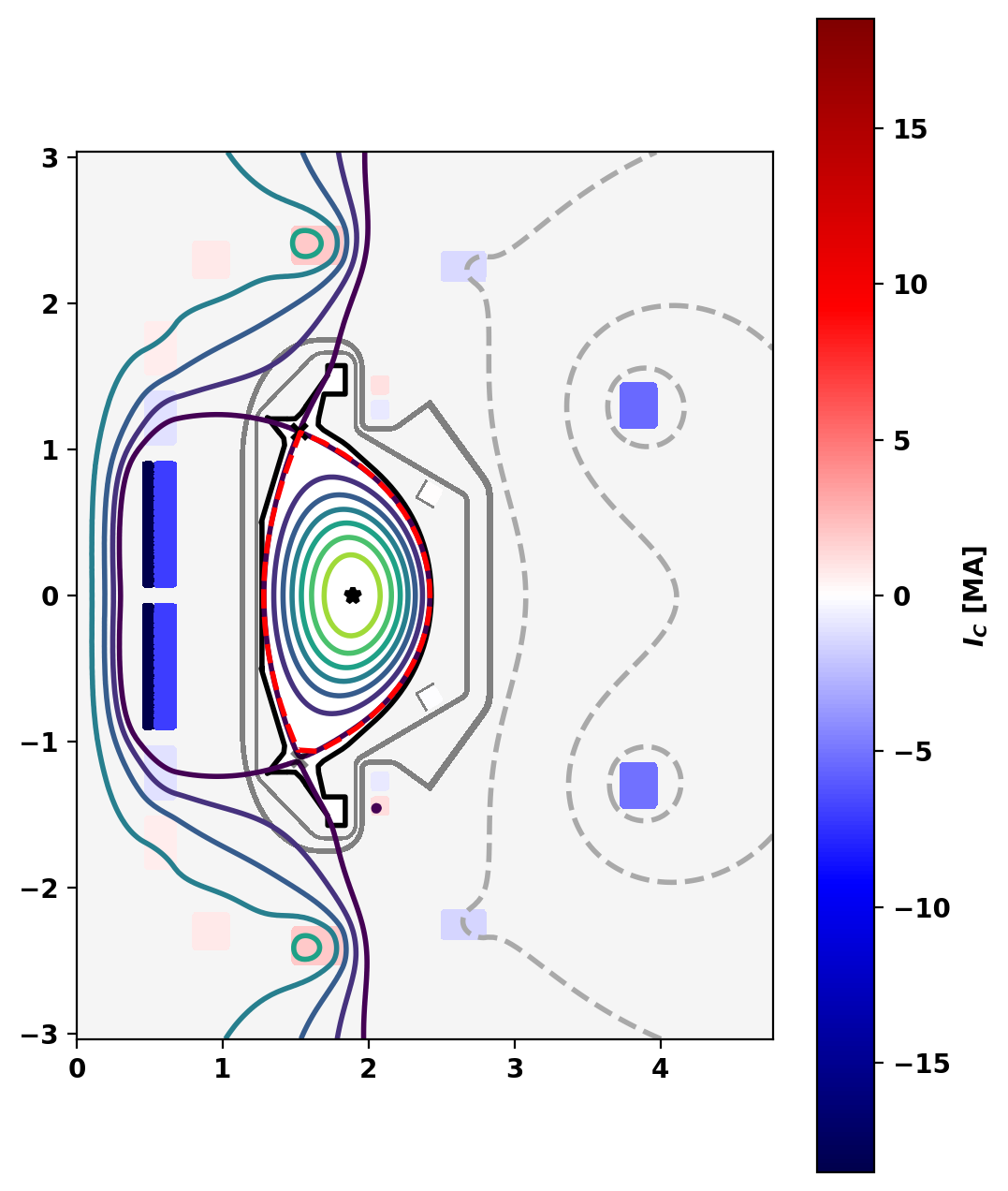
Basic parameters can be displayed using the print_info() method. For access to these quantities as variables instead the get_stats() can be used.
The final coil currents can also be retrieved using the get_coil_currents() method. Here, we print the deviation of the TokaMaker currents from the desired target currents set above. TokaMaker reports the current per turn; multiplying by the turn count from the device description gives the total A-turns in each coil.
Equilibrium Statistics:
  Topology                =   Diverted
  Toroidal Current [A]    =    8.7000E+06
  Current Centroid [m]    =    1.843  0.001
  Magnetic Axis [m]       =    1.891  0.001
  Elongation              =    1.969 (U:  1.992, L:  1.946)
  Triangularity           =    0.559 (U:  0.569, L:  0.550)
  Plasma Volume [m^3]     =   20.222
  q_0, q_95               =    0.950  3.168
  Plasma Pressure [Pa]    =   Axis:  2.5952E+06, Peak:  2.5952E+06
  Stored Energy [J]       =    1.8205E+07
  <Beta_pol> [%]          =   36.6018
  <Beta_tor> [%]          =    1.0218
  <Beta_n>   [%]          =    0.8110
  Diamagnetic flux [Wb]   =    2.3655E-01
  Toroidal flux [Wb]      =    2.3119E+01
  l_i                     =    1.2970

  Coil             I [kA]  Target [kA]
  CS1UI:           -66.14         0.00
  CS1UO:           -52.49         0.00
  CS1LI:           -65.75         0.00
  CS1LO:           -52.16         0.00
  CS2U:            -25.75         0.00
  CS2L:            -25.78         0.00
  CS3U:             15.71         0.00
  CS3L:             14.94         0.00
  PF1U:             31.21         0.00
  PF1L:             30.79         0.00
  PF2U:             64.82         0.00
  PF2L:             64.58         0.00
  PF3U:            -39.78         0.00
  PF3L:            -42.67         0.00
  PF4U:           -178.74         0.00
  PF4L:           -173.18         0.00
  DV1U:             44.47         0.00
  DV1L:             46.67         0.00
  DV2U:            -29.42         0.00
  DV2L:            -30.68         0.00
  VS1U:              0.29         0.00
  VS1L:             -0.46         0.00
Here, we use get_profiles() and get_q()to obtain the profiles of our equilibrium and compare them to the profiles of the target gEQDSK. Note the gEQDSK curves are plotted without the sign flip used in the ARC example, for the reason given above.
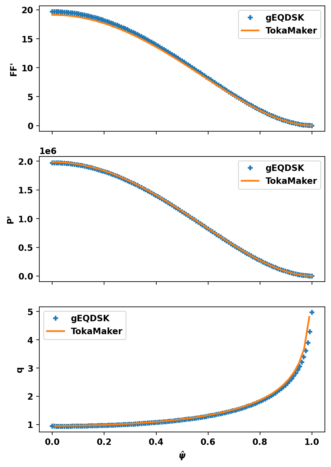
  Quantity                  TokaMaker       gEQDSK
  Ip [MA]                        8.70         8.70
  R_axis [m]                    1.891        1.890
  kappa                         1.969        1.955
  q_0                           0.950        0.939
  q_95                          3.168        3.008
  p_axis [MPa]                   2.60         2.60

  Topology: Diverted (gEQDSK: double null)
 1.17.0