This is based on the open source SPARC device description published by Commonwealth Fusion Systems (CFS) in the SPARCPublic repository. SPARC is a compact high-field tokamak ( \(R_0 = 1.85\) m, \(B_0 = 12.2\) T); the physics basis is described in the special series of seven papers in the Journal of Plasma Physics (2020), starting with Creely et al, "Overview of the SPARC tokamak", J. Plasma Phys. 86(5), 865860502. https://doi.org/10.1017/S0022377820001257
All files available on GitHub at: https://github.com/cfs-energy/SPARCPublic/
- Note
- as CFS states in the repository, the device description is not an accurate description of the geometry of SPARC. It is based on SPARC, but details protected by CFS' intellectual property have been removed or changed — in particular the division of the coils into turns is replaced by toy data. It is intended as a realistic example of an IMAS-schema geometry description for building example workflows, which is how we use it here.
import os
import sys
import json
import numpy as np
import matplotlib.pyplot as plt
from scipy.spatial import ConvexHull
from matplotlib.path import Path
plt.rcParams['figure.figsize']=(6,6)
plt.rcParams['font.weight']='bold'
plt.rcParams['axes.labelweight']='bold'
plt.rcParams['lines.linewidth']=2
plt.rcParams['lines.markeredgewidth']=2
%matplotlib inline
%config InlineBackend.figure_format = "retina"
Load TokaMaker library
To load the TokaMaker python module we need to tell python where to the module is located. This can be done either through the PYTHONPATH environment variable or using within a script using sys.path.append() as below, where we look for the environement variable OFT_ROOTPATH to provide the path to where the OpenFUSIONToolkit is installed (/Applications/OFT on macOS).
For meshing we will use the gs_Domain class to build a 2D triangular grid suitable for Grad-Shafranov equilibria. This class uses the triangle code through a python wrapper.
tokamaker_python_path = os.getenv('OFT_ROOTPATH')
if tokamaker_python_path is not None:
sys.path.append(os.path.join(tokamaker_python_path,'python'))
Load geometry information
The geometry information (e.g. bounding curves for vacuum vessels) is loaded from a JSON file available in the SPARCPublic repository. The cell below reads the file directly from the repository over HTTP each time the notebook is run, so no copy of the device description is kept locally and the notebook always tracks the published version.
The SPARC description follows the IMAS/OMAS data schema (it was written with the OMAS library). CFS ship a plot.py alongside it that demonstrates the access patterns; we reproduce those here with the plain json library so the notebook has no extra dependencies. The fields we need are:
- wall.description_2d[0]: a block description of the vessel (vessel.type.index == 1), holding closed outlines of the structural sections of the inner and outer wall, plus limiter.unit[0].outline, the closed limiter (plasma-facing) contour
- wall.description_2d[1]: an annular description of the same two vessel walls (vessel.type.index == 0), giving outline_inner / outline_outer and a resistivity for each. This is the form gs_Domain.add_annulus wants, so it is what we use below
- pf_active.coil: the 22 PF/CS/DV/VS coils. Each coil is a list of elements whose geometry is an annulus — i.e. each turn is a circular filament at (r, z) with radius_outer (radius_inner is zero throughout), rather than a rectangular grid of filaments
- pf_passive.loop: the two passive shielding covers for the in-vessel vertical stability coils, each a closed outline polygon with a resistivity
import urllib.request
_SPARC_RAW = 'https://raw.githubusercontent.com/cfs-energy/SPARCPublic/main/DeviceDescription'
def fetch_json(filename):
"""Read a JSON file straight from the SPARCPublic repo, without writing it to disk."""
print(f'Fetching {filename} from SPARCPublic...', end=' ', flush=True)
with urllib.request.urlopen(f'{_SPARC_RAW}/{filename}') as resp:
data = json.load(resp)
print('done.')
return data
mach = fetch_json('OS_SPARC_Device_Description.json')
print('Machine:', mach['dataset_description']['data_entry']['machine'],
'| IMAS DD version:', mach['dataset_description']['dd_version'])
print('R0 =', mach['summary']['global_quantities']['r0']['value'], 'm')
Fetching OS_SPARC_Device_Description.json from SPARCPublic... done.
Machine: SPARC | IMAS DD version: 3.41.0
R0 = 1.8495 m
Define coil array
In the SPARC file the turns are circular filaments (geometry.annulus), and two of the coils — the in-vessel vertical stability coils VS1U/VS1L — are tilted so that they follow the outboard vessel wall. An axis-aligned bounding rectangle around a tilted coil would spill outside the winding pack and, as it happens, cut straight through the VS coil covers.
We therefore take the convex hull of the filament circles (each circle sampled by a polygon of nseg points) as the coil boundary. This reduces to the expected octagonal-cornered box for the axis-aligned CS/PF/DV coils and correctly follows the tilt of the VS coils. The turn count is taken from the number of filament elements.
def coil_boundary(coil_elements, nseg=16):
"""Return the convex hull of a coil's filament circles, and the turn count.
Each element is an IMAS "annulus": a circular filament at (r, z) with an outer
radius. The hull of those circles bounds the winding pack, and unlike a bounding
rectangle it stays tight around coils that are tilted (VS1U/VS1L).
"""
pts = []
for el in coil_elements:
ann = el['geometry']['annulus']
theta = np.linspace(0.0, 2.0*np.pi, nseg, endpoint=False)
pts.append(np.column_stack((ann['r'] + ann['radius_outer']*np.cos(theta),
ann['z'] + ann['radius_outer']*np.sin(theta))))
pts = np.vstack(pts)
hull = pts[ConvexHull(pts).vertices]
return hull, len(coil_elements)
coil_data = {}
plt.figure()
for coil in mach['pf_active']['coil']:
hull, n = coil_boundary(coil['element'])
turns_signed = sum(el['turns_with_sign'] for el in coil['element'])
coil_data[coil['name']] = dict(hull=hull, n_filaments=n, turns_signed=turns_signed)
plt.fill(hull[:,0], hull[:,1], facecolor='none', edgecolor='k', lw=1)
plt.gca().set_aspect('equal')
plt.xlabel('R (m)')
plt.ylabel('Z (m)')
plt.title('PF coil winding pack boundaries')
plt.show()
coil_name = list(coil_data.keys())
coil_nturns = [coil_data[c]['n_filaments'] for c in coil_name]
for name in coil_name:
c = coil_data[name]
r = c['hull'][:,0]; z = c['hull'][:,1]
print(f"{name:<8} r=[{r.min():.4f}, {r.max():.4f}] z=[{z.min():+.4f}, {z.max():+.4f}]"
f" n={c['n_filaments']:>3} turns_with_sign={c['turns_signed']:+.0f}")
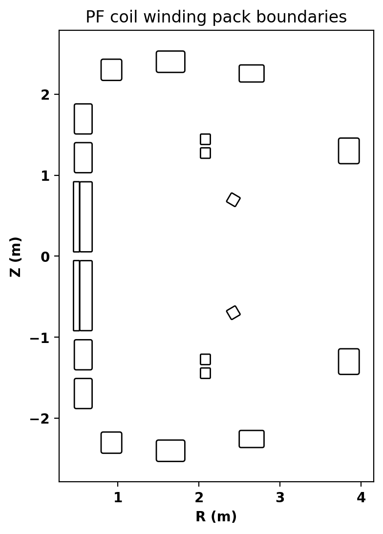
CS1UI     r=[0.4518, 0.5264]  z=[+0.0534, +0.9196]  n=280  turns_with_sign=+280
CS1UO     r=[0.5288, 0.6824]  z=[+0.0545, +0.9185]  n=135  turns_with_sign=+135
CS1LI     r=[0.4518, 0.5264]  z=[-0.9196, -0.0534]  n=280  turns_with_sign=+280
CS1LO     r=[0.5288, 0.6824]  z=[-0.9185, -0.0545]  n=135  turns_with_sign=+135
CS2U      r=[0.4622, 0.6818]  z=[+1.0305, +1.4015]  n= 40  turns_with_sign=+40
CS2L      r=[0.4622, 0.6818]  z=[-1.4015, -1.0305]  n= 40  turns_with_sign=+40
CS3U      r=[0.4622, 0.6818]  z=[+1.5085, +1.8795]  n= 40  turns_with_sign=+40
CS3L      r=[0.4622, 0.6818]  z=[-1.8795, -1.5085]  n= 40  turns_with_sign=+40
PF1U      r=[0.7926, 1.0474]  z=[+2.1690, +2.4310]  n= 25  turns_with_sign=+25
PF1L      r=[0.7926, 1.0474]  z=[-2.4310, -2.1690]  n= 25  turns_with_sign=+25
PF2U      r=[1.4741, 1.8259]  z=[+2.2682, +2.5318]  n= 30  turns_with_sign=+30
PF2L      r=[1.4741, 1.8259]  z=[-2.5318, -2.2682]  n= 30  turns_with_sign=+30
PF3U      r=[2.4969, 2.8031]  z=[+2.1496, +2.3603]  n= 35  turns_with_sign=+35
PF3L      r=[2.4969, 2.8031]  z=[-2.3603, -2.1496]  n= 35  turns_with_sign=+35
PF4U      r=[3.7226, 3.9774]  z=[+1.1420, +1.4580]  n= 30  turns_with_sign=+30
PF4L      r=[3.7226, 3.9774]  z=[-1.4580, -1.1420]  n= 30  turns_with_sign=+30
DV1U      r=[2.0187, 2.1403]  z=[+1.3786, +1.5074]  n= 25  turns_with_sign=+25
DV1L      r=[2.0187, 2.1403]  z=[-1.5074, -1.3786]  n= 25  turns_with_sign=+25
DV2U      r=[2.0187, 2.1403]  z=[+1.2086, +1.3374]  n= 25  turns_with_sign=+25
DV2L      r=[2.0187, 2.1403]  z=[-1.3374, -1.2086]  n= 25  turns_with_sign=+25
VS1U      r=[2.3416, 2.5074]  z=[+0.6141, +0.7799]  n= 25  turns_with_sign=+25
VS1L      r=[2.3416, 2.5074]  z=[-0.7799, -0.6141]  n= 25  turns_with_sign=-25
Here we check the resistivity of each element in the json, printing the results to the notebook. SPARC's description carries two conducting structures: the double-walled vacuum vessel (given in both block and annular form) and the two passive covers over the in-vessel VS coils.
for i, element in enumerate(mach['wall']['description_2d']):
print(f"[{i}]", element['type'])
if 'vessel' in element.keys():
print(f" vessel type: {element['vessel']['type']['description']}")
print(f" {len(element['vessel']['unit'])} items:")
for item in element['vessel']['unit']:
try:
print(' -- ', item['name'], item['annular'].keys())
print(' ', 'Resistivity:', item['annular']['resistivity'])
except KeyError:
print(' -- ', item['name'], f"({len(item['element'])} blocks)")
print(' ', 'Resistivity:', item['element'][0]['resistivity'])
print()
print('pf_passive:')
for loop in mach['pf_passive']['loop']:
print(' -- ', loop['name'])
print(' ', 'Resistivity:', loop['resistivity'])
[0] {'description': 'Single limiter surface and block element vessel', 'index': 0}
    vessel type: Block description of the vessel
    2 items:
 --  inner wall (8 blocks)
     Resistivity: 8e-07
 --  outer wall (8 blocks)
     Resistivity: 8e-07
[1] {'description': 'Annular description of vessel (limiter field not filled)', 'index': -1}
    vessel type: Annular description of the vessel
    2 items:
 --  Vacuum vessel inner wall dict_keys(['outline_inner', 'outline_outer', 'resistivity'])
     Resistivity: 8e-07
 --  Vacuum vessel outer wall dict_keys(['outline_inner', 'outline_outer', 'resistivity'])
     Resistivity: 8e-07

pf_passive:
 --  Cover upper vertical stability coil
     Resistivity: 8e-07
 --  Cover lower vertical stability coil
     Resistivity: 8e-07
Set mesh resolution for each region
First we define some target sizes to set the resolution in out grid. These variables will be used later and represent the target edge size within a given region, where units are in meters. In this case we are using a fairly coarse resolution for speed, but you can increase it for fidelity if needed.
plasma_res = 0.05
coil_res = 0.03
vv_res = 0.02
vac_res = 0.06
cover_res = 0.008
Define regions and attributes
We now create and define the various logical mesh regions. In the SPARC case we have 7 kinds of region:
- air: The region outside the outer vacuum vessel, which is not actually air in a superconducting device like SPARC but we use this terminology for commonality with present research devices. This is the outer bounding region and holds all of the CS, PF and DV coils
- vac_vessel: The vacuum gap between the inner and outer vacuum vessel walls
- vac_inner: The vacuum region inside the vacuum vessel but outside the limiter, which holds the in-vessel VS coils and their covers
- plasma: The region inside the limiter where the plasma will exist
- vessel_inner: The inner vacuum vessel wall
- vessel_outer: The outer vacuum vessel wall
- vs_cover_upper / vs_cover_lower: (optional) The passive shielding covers over the in-vessel VS coils
- coil: The 22 coils
Two SPARC-specific points are worth calling out, both of which follow from the geometry rather than from any choice we make:
- The limiter is a distinct contour well inside the vessel, so the plasma region is bounded by the limiter and a separate vacuum region (vac_inner) sits between the limiter and the inner vessel wall. In the ARC file the plasma region ran all the way to the inner vessel wall.
- The DV1/DV2 divertor coils sit in the re-entrant divertor pocket, which is topologically outside the vessel, so they belong to the air region despite visually appearing to be tucked inside the machine. Only VS1U/VS1L are genuinely in-vessel. Rather than hard-code this we assign each coil to its parent region by testing which contour contains it.
for i, dsc in enumerate(mach['wall']['description_2d']):
if 'vessel' in dsc and dsc['vessel']['type']['index'] == 0:
i_annular = i
vv_units = mach['wall']['description_2d'][i_annular]['vessel']['unit']
def annular_contours(unit):
ann = unit['annular']
inner = np.column_stack((ann['outline_inner']['r'], ann['outline_inner']['z']))
outer = np.column_stack((ann['outline_outer']['r'], ann['outline_outer']['z']))
return inner, outer
vv_inner_inner, vv_inner_outer = annular_contours(vv_units[0])
vv_outer_inner, vv_outer_outer = annular_contours(vv_units[1])
limiter_unit = mach['wall']['description_2d'][0]['limiter']['unit'][0]
limiter_contour = np.column_stack((limiter_unit['outline']['r'], limiter_unit['outline']['z']))
path_vv_inner = Path(vv_inner_inner)
path_vv_outer = Path(vv_outer_inner)
for name in coil_name:
centroid = coil_data[name]['hull'].mean(axis=0)
if path_vv_inner.contains_point(centroid):
coil_data[name]['parent'] = 'vac_inner'
elif path_vv_outer.contains_point(centroid):
coil_data[name]['parent'] = 'vac_vessel'
else:
coil_data[name]['parent'] = 'air'
for parent in ('air', 'vac_vessel', 'vac_inner'):
members = [n for n in coil_name if coil_data[n]['parent'] == parent]
print(f'{parent:<11}: {len(members):>2} coils {members}')
air        : 20 coils  ['CS1UI', 'CS1UO', 'CS1LI', 'CS1LO', 'CS2U', 'CS2L', 'CS3U', 'CS3L', 'PF1U', 'PF1L', 'PF2U', 'PF2L', 'PF3U', 'PF3L', 'PF4U', 'PF4L', 'DV1U', 'DV1L', 'DV2U', 'DV2L']
vac_vessel :  0 coils  []
vac_inner  :  2 coils  ['VS1U', 'VS1L']
gs_mesh = gs_Domain()
gs_mesh.define_region('air', vac_res, 'boundary')
gs_mesh.define_region('vac_vessel', vac_res, 'vacuum')
gs_mesh.define_region('vac_inner', vac_res, 'vacuum')
gs_mesh.define_region('plasma', plasma_res, 'plasma')
gs_mesh.define_region('vessel_inner', vv_res, 'conductor', vv_units[0]['annular']['resistivity'], allow_xpoints=True)
gs_mesh.define_region('vessel_outer', vv_res, 'conductor', vv_units[1]['annular']['resistivity'], allow_xpoints=True)
include_VS_covers = True
cover_names = {}
for loop in mach['pf_passive']['loop']:
cover_names[loop['name']] = 'vs_cover_upper' if 'upper' in loop['name'] else 'vs_cover_lower'
if include_VS_covers:
for loop in mach['pf_passive']['loop']:
gs_mesh.define_region(cover_names[loop['name']], cover_res, 'conductor',
loop['resistivity'], allow_xpoints=True)
for name in coil_name:
gs_mesh.define_region(name, coil_res, 'coil', nTurns=coil_data[name]['n_filaments'])
Define geometry for region boundaries
Once the region types and properties are defined we now define the geometry of the mesh using shapes and references to the defined regions.
Working outward from the plasma: the limiter bounds the plasma; the inner vessel wall is an annulus separating vac_inner from vac_vessel; the outer vessel wall is an annulus separating vac_vessel from air. The coils and VS covers are then dropped into whichever region contains them.
gs_mesh.add_polygon(limiter_contour, 'plasma', parent_name='vac_inner')
gs_mesh.add_annulus(vv_inner_inner, 'vac_inner', vv_inner_outer, 'vessel_inner', parent_name='vac_vessel')
gs_mesh.add_annulus(vv_outer_inner, 'vac_vessel', vv_outer_outer, 'vessel_outer', parent_name='air')
if include_VS_covers:
for loop in mach['pf_passive']['loop']:
outline = loop['element'][0]['geometry']['outline']
cover_contour = np.column_stack((outline['r'], outline['z']))
gs_mesh.add_polygon(cover_contour, cover_names[loop['name']], parent_name='vac_inner')
for name in coil_name:
gs_mesh.add_polygon(coil_data[name]['hull'], name, parent_name=coil_data[name]['parent'])
Warning: Sliver (angle=18.5) detected at point 15 (1.305519082, 1.219477963)
Warning: Sliver (angle=18.5) detected at point 163 (1.305519082, -1.219477963)
Plot topology
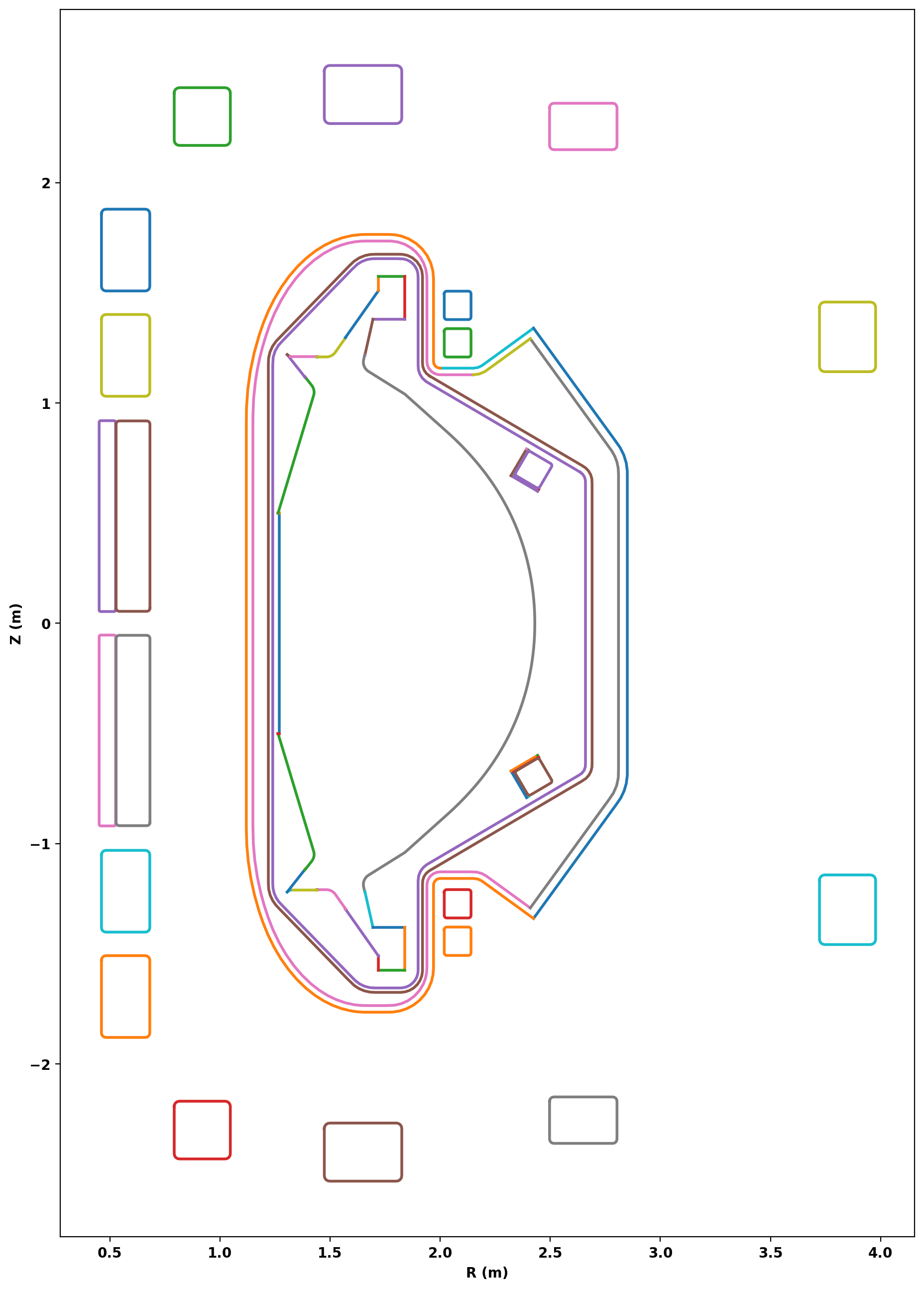
After defining the logical and physical topology we can now plot the curves within the definitions to double check everything is in the right place. In cases where curves appear to cross eachother (as with the VS coils and their covers) one should zoom in to ensure no crossings exist. Because we bound each coil by the convex hull of its filaments rather than by an axis-aligned rectangle, the tilted VS coils clear their covers and no curves needed to be moved for this example.
fig, ax = plt.subplots(1,1, figsize=(20,16))
gs_mesh.plot_topology(fig,ax)
Create mesh
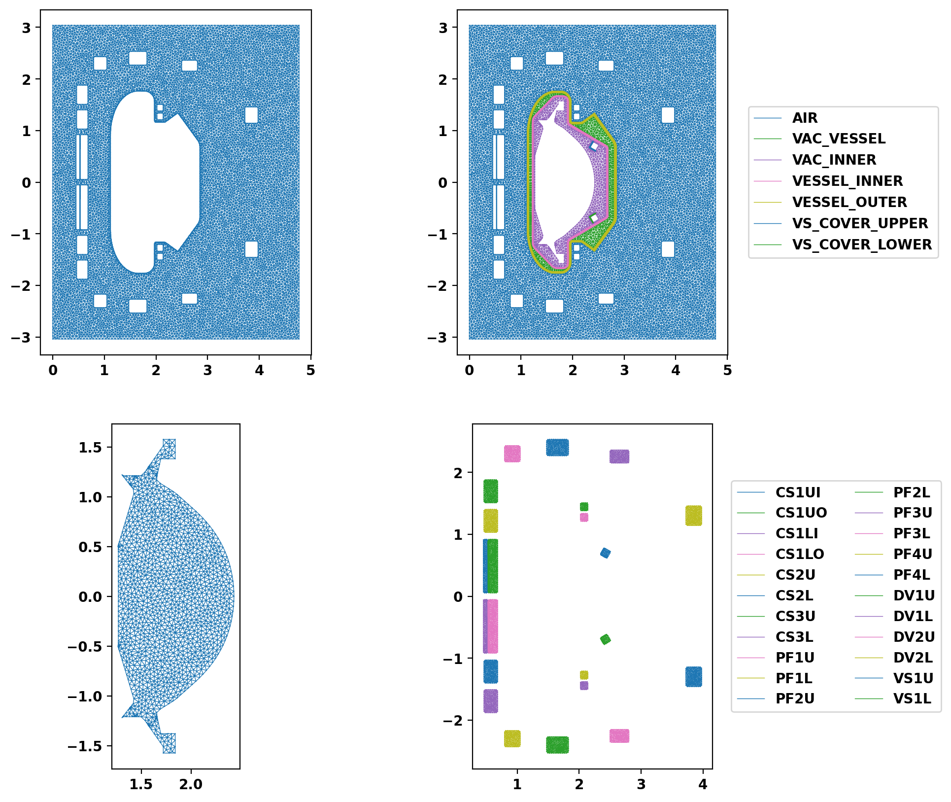
Now we generate the actual mesh using the build_mesh method. Additionally, since coil and conductor regions are defined, the get_coils and get_conductors methods should also be called to get descriptive dictionaries for later use in TokaMaker. This step may take a few moments as triangle generates the mesh.
The "small feature" warnings below come from the fine structure of the limiter contour in the divertor region, which is resolved more finely than our target plasma edge length; they are informational.
mesh_pts, mesh_lc, mesh_reg = gs_mesh.build_mesh()
coil_dict = gs_mesh.get_coils()
cond_dict = gs_mesh.get_conductors()
Assembling regions:
Warning: Small feature (dl=5.00E-03) detected at point 2 (1.269, 0.5)
Warning: Small feature (dl=1.00E-03) detected at point 13 (1.3874270979999999, 1.117237672)
Warning: Small feature (dl=1.73E-02) detected at point 15 (1.305519082, 1.219477963)
Warning: Small feature (dl=1.00E-03) detected at point 17 (1.4407, 1.21)
Warning: Small feature (dl=1.00E-03) detected at point 28 (1.5708, 1.2964)
Warning: Small feature (dl=1.02E-03) detected at point 35 (1.6585, 1.2177)
Warning: Small feature (dl=1.02E-03) detected at point 142 (1.6575, -1.2179)
Warning: Small feature (dl=1.00E-03) detected at point 149 (1.57, -1.297)
Warning: Small feature (dl=1.00E-03) detected at point 160 (1.4407, -1.209)
Warning: Small feature (dl=1.73E-02) detected at point 162 (1.32, -1.21)
Warning: Small feature (dl=1.00E-03) detected at point 164 (1.38664191, -1.116618414)
Warning: Small feature (dl=5.00E-03) detected at point 175 (1.264, -0.5)
  # of unique points    = 3225
  # of unique segments  = 80
Generating mesh with Triangle:
  # of points  = 18989
  # of cells   = 37616
  # of regions = 30
Plot resulting regions and grid
We now plot the mesh by region to inspect proper generation.
fig, ax = plt.subplots(2,2,figsize=(10,10))
ax[0,0].triplot(mesh_pts[:,0],mesh_pts[:,1],mesh_lc[mesh_reg==2,:],lw=0.5)
ax[1,0].triplot(mesh_pts[:,0],mesh_pts[:,1],mesh_lc[mesh_reg==1,:],lw=0.5)
for key, cond in cond_dict.items():
ax[0,1].triplot(mesh_pts[:,0],mesh_pts[:,1],mesh_lc[mesh_reg==cond['reg_id'],:],lw=0.5,label=key)
for key, coil in coil_dict.items():
ax[1,1].triplot(mesh_pts[:,0],mesh_pts[:,1],mesh_lc[mesh_reg==coil['reg_id'],:],lw=0.5,label=key)
for ax_tmp in ax.flatten():
ax_tmp.set_aspect('equal','box')
ax[0,1].legend(bbox_to_anchor=(1.05,0.5), loc='center left')
_ = ax[1,1].legend(bbox_to_anchor=(1.05,0.5), ncol=2, loc='center left')
plt.show()
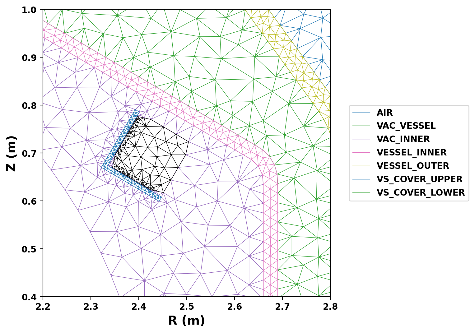
Zooming in on the outboard midplane shows the in-vessel VS coil sitting between the limiter and the inner vessel wall, with its passive cover in front of it.
fig, ax = plt.subplots(1,1,figsize=(8,6))
for key, cond in cond_dict.items():
print(key)
ax.triplot(mesh_pts[:,0],mesh_pts[:,1],mesh_lc[mesh_reg==cond['reg_id'],:],lw=0.5,label=key)
for key, coil in coil_dict.items():
ax.triplot(mesh_pts[:,0],mesh_pts[:,1],mesh_lc[mesh_reg==coil['reg_id'],:],lw=0.5,color='k')
ax.set_aspect('equal','box')
ax.set_xlim(2.2,2.8)
ax.set_ylim(0.4,1.0)
ax.legend(bbox_to_anchor=(1.05,0.5), loc='center left')
ax.set_xlabel('R (m)', fontsize=14)
ax.set_ylabel('Z (m)', fontsize=14)
plt.show()
AIR
VAC_VESSEL
VAC_INNER
VESSEL_INNER
VESSEL_OUTER
VS_COVER_UPPER
VS_COVER_LOWER
Save mesh for later use
As generation of the mesh often takes comparable, or longer, time compare to runs in TokaMaker it is useful to separate generation of the mesh into a different script as demonstrated here. The method save_gs_mesh can be used to save the resulting information for later use. This is done using and an HDF5 file through the h5py library.
fname = ''
save_gs_mesh(mesh_pts, mesh_lc, mesh_reg, coil_dict, cond_dict, f"sparc_public_mesh{fname}.h5")
 1.17.0