In this example we demonstrate how to compute a current potential from a given B-norm on a toroidal surface. This has application to compute eddy current and sensor reponse to plasma modes.

Note: Running this example requires the h5py python package, which is installable using pip or other standard methods.

import struct
import sys
import os
import h5py
import numpy as np
import matplotlib.pyplot as plt
import matplotlib as mpl
plt.rcParams['figure.figsize']=(6,6)
plt.rcParams['font.weight']='bold'
plt.rcParams['axes.labelweight']='bold'
plt.rcParams['lines.linewidth']=2
plt.rcParams['lines.markeredgewidth']=2
%matplotlib inline
%config InlineBackend.figure_format = "retina"

Load ThinCurr library

To load the ThinCurr python module we need to tell python where to the module is located. This can be done either through the PYTHONPATH environment variable or within a script using sys.path.append() as below, where we look for the environement variable OFT_ROOTPATH to provide the path to where the OpenFUSIONToolkit is installed (/Applications/OFT for binaries on macOS).

thincurr_python_path = os.getenv('OFT_ROOTPATH')
if thincurr_python_path is not None:
    sys.path.append(os.path.join(thincurr_python_path,'python'))
from OpenFUSIONToolkit.ThinCurr import ThinCurr
from OpenFUSIONToolkit.ThinCurr.meshing import write_ThinCurr_mesh, build_torus_bnorm_grid, build_periodic_mesh, write_periodic_mesh
from OpenFUSIONToolkit.util import build_XDMF

Create 3D mode model

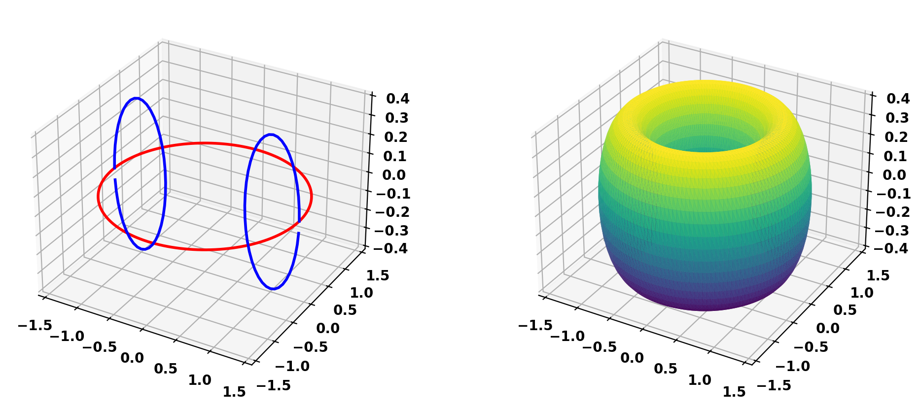
In most cases the mode will be imported and/or converted from another tool (eg. DCON). However, in this case we will generate a simple mode shape with fixed toroidal and poloidal mode number for a simple torus. Using a simple helper function we define an n=2, m=3 mode on an R=1.0 m, a=0.4 m torus.

def create_circular_bnorm(filename,R0,Z0,a,n,m,npts=200):
    theta_vals = np.linspace(0.0,2*np.pi,npts,endpoint=False)
    with open(filename,'w+') as fid:
        fid.write('{0} {1}\n'.format(npts,n))
        for theta in theta_vals:
            fid.write('{0} {1} {2} {3}\n'.format(
                R0+a*np.cos(theta),
                Z0+a*np.sin(theta),
                np.cos(m*theta),
                np.sin(m*theta)
            ))
# Create n=2, m=3 mode
create_circular_bnorm('tCurr_mode.dat',1.0,0.0,0.4,2,3)

Generate mesh and ThinCurr input from mode file

We can now create a ThinCurr model from the mode definition file by using build_torus_bnorm_grid() to build a uniform grid over one toroidal field period and build_periodic_mesh() to build a mesh from the resulting grid. The result is a ThinCurr model, including periodicity mapping information (r_map), and the normal field at each mesh vertex for the Real and Imaginary components of the mode (bnorm).

ntheta = 40
nphi = 80
r_grid, bnorm, nfp = build_torus_bnorm_grid('tCurr_mode.dat',ntheta,nphi,resample_type='theta',use_spline=False)
lc_mesh, r_mesh, tnodeset, pnodesets, r_map = build_periodic_mesh(r_grid,nfp)

Loading toroidal plasma mode
  filename = tCurr_mode.dat
  N        = 2
  # of pts = 200
  R0       = (1.0000E+00, -1.7087E-17)
  Mode pair sums -7.6050E-15 -2.9976E-15

Plot resulting mesh

fig = plt.figure(figsize=(12,5))
ax = fig.add_subplot(1,2,1, projection='3d')
ax.plot(r_mesh[tnodeset,0], r_mesh[tnodeset,1], r_mesh[tnodeset,2], c='red')
for pnodeset in pnodesets:
    ax.plot(r_mesh[pnodeset,0], r_mesh[pnodeset,1], r_mesh[pnodeset,2], c='blue')
 
ax = fig.add_subplot(1,2,2, projection='3d')
_ = ax.plot_trisurf(r_mesh[:,0], r_mesh[:,1], r_mesh[:,2], triangles=lc_mesh, cmap='viridis')

Save model to HDF5 format

write_periodic_mesh('thincurr_mode.h5', r_mesh, lc_mesh+1, np.ones((lc_mesh.shape[0],)),

tnodeset, pnodesets, pmap=r_map, nfp=nfp, include_closures=True)

Saving mesh: thincurr_mode.h5

Compute mode-equivalent current distribution

Setup ThinCurr model

We now create a ThinCurr instance to use for equilibrium calculations. Once created, we setup the model from an existing HDF5 and XML mesh definition using setup_model(). We also initialize I/O for this model using setup_io() to enable output of plotting files for 3D visualization in VisIt or Paraview.

In this case we specify a plasma directory to use for saving I/O files to keep things separate for the other cases to be run in ThinCurr Python Example: Compute frequency-response in a torus.

Note: A warning will be generated that no XML node was found and a default resistivity value is being used. This is OK as we will not use the resitivity matrix in this example.

tw_mode = ThinCurr(nthreads=4)
tw_mode.setup_model(mesh_file='thincurr_mode.h5')
tw_mode.setup_io(basepath='plasma/')

#----------------------------------------------
Open FUSION Toolkit Initialized
Development branch:   main
Revision id:          8440e61
Parallelization Info:
  Not compiled with MPI
  # of OpenMP threads =    4
Fortran input file    = oftpyin                                                                         
XML input file        = none                                                                            
Integer Precisions    =    4   8
Float Precisions      =    4   8  16
Complex Precisions    =    4   8
LA backend            = native
#----------------------------------------------


Creating thin-wall model
 Orientation depth =       12640
  Loading V(t) driver coils
  Loading I(t) driver coils

  # of points    =         6320
  # of edges     =        18960
  # of cells     =        12640
  # of holes     =            3
  # of Vcoils    =            0
  # of closures  =            2
  # of Icoils    =            0

  Building holes


WARNING: Unable to find "thincurr" XML node
WARNING: No "thincurr" XML node, using "eta=mu0" for all regions

Compute self-inductance matrix

With the model setup, we can now compute the self-inductance matrix. A numpy version of the self-inductance matrix will be stored at tw_plate.Lmat. For this case we will use the self-inductance to convert between the surface flux \(\Phi\) corresponding to the normal field computed above (bnorm) and an equivalent surface current

\(\textrm{L} I = \Phi\)

Note: For larger models calculating the self-inductance may take some time due to the \(N^2\) interaction of the elements (see ThinCurr Example: Using HODLR approximation for more information).

While model definition above handles most of the periodicity, however as pointed out we still end up with nfp copies of the poloidal hole. So if nfp>1 we must condense the self-inductance matrix by summing values over these rows/columns.

Finally, we compute \(\textrm{L}^{-1}\).

tw_mode.compute_Lmat()
# Condense model to single mode period
if nfp > 1:
    nelems_new = tw_mode.Lmat.shape[0]-nfp+1
    Lmat_new = np.zeros((nelems_new,nelems_new))
    Lmat_new[:-1,:-1] = tw_mode.Lmat[:-nfp,:-nfp]
    Lmat_new[:-1,-1] = tw_mode.Lmat[:-nfp,-nfp:].sum(axis=1)
    Lmat_new[-1,:-1] = tw_mode.Lmat[-nfp:,:-nfp].sum(axis=0)
    Lmat_new[-1,-1] = tw_mode.Lmat[-nfp:,-nfp:].sum(axis=None)
else:
    Lmat_new = tw_mode.Lmat
# Get inverse
Linv = np.linalg.inv(Lmat_new)

 Building element<->element self inductance matrix
     Time = 19s

Compute currents from fluxes and save

Now we can compute the equivalent currents for the Real and Imaginary component of normal field \(B_n\) from above. To do this we need to convert to flux \(\Phi\) by scaling the field by the area of each vertex using scale_va(). As the flux is only given on points we need to supplement those values to the full system size by adding the toroidal and poloidal holes (copying if necessary for nfp>1). As a single closure is also needed, we remove the first entry of flux_flat as well.

bnorm_flat = bnorm.reshape((2,bnorm.shape[1]*bnorm.shape[2]))
# Get surface flux from normal field
flux_flat = bnorm_flat.copy()
flux_flat[0,r_map] = tw_mode.scale_va(bnorm_flat[0,r_map])
flux_flat[1,r_map] = tw_mode.scale_va(bnorm_flat[1,r_map])
if nfp > 1:
    tw_mode.save_scalar(bnorm_flat[0,r_map],'Bn_c')
    tw_mode.save_scalar(bnorm_flat[1,r_map],'Bn_s')
    output = np.zeros((2,nelems_new+nfp-1))
    for j in range(2):
        output[j,:nelems_new] = np.dot(Linv,np.r_[flux_flat[j,1:-bnorm.shape[2]],0.0,0.0])
        output[j,-nfp+1:] = output[j,-nfp]
else:
    tw_mode.save_scalar(bnorm_flat[0,:],'Bn_c')
    tw_mode.save_scalar(bnorm_flat[1,:],'Bn_s')
    output = np.zeros((2,tw_mode.Lmat.shape[0]))
    for j in range(2):
        output[j,:] = np.dot(Linv,np.r_[flux_flat[j,1:],0.0,0.0])
tw_mode.save_current(output[0,:],'Jc')
tw_mode.save_current(output[1,:],'Js')
tw_mode.build_XDMF()

Removing old Xdmf files
Creating output files

Plot current potential and mode shape

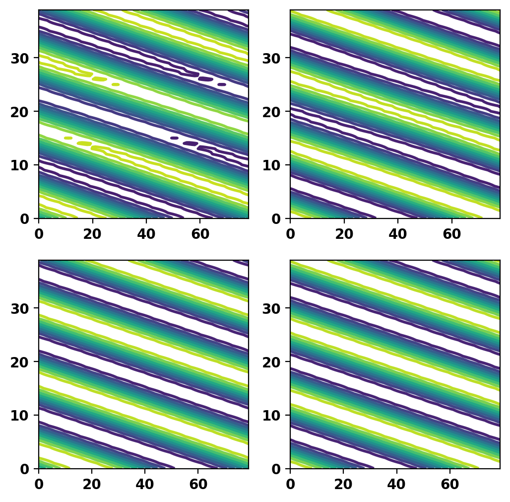
We now plot the resulting current potential (top) and mode shape (bottom) over a single toroidal mode period to show how the fields are related and ensure no errors.

fig, ax = plt.subplots(2,2)
if nfp > 1:
    ax[0,0].contour(np.r_[0.0,output[0,:-nfp-1]].reshape((nphi-1,ntheta)).transpose(),10)
    ax[0,1].contour(np.r_[0.0,output[1,:-nfp-1]].reshape((nphi-1,ntheta)).transpose(),10)
else:
    ax[0,0].contour(np.r_[0.0,output[0,:-nfp-1]].reshape((nphi,ntheta)).transpose(),10)
    ax[0,1].contour(np.r_[0.0,output[1,:-nfp-1]].reshape((nphi,ntheta)).transpose(),10)
ax[1,0].contour(bnorm[0,:,:].transpose(),10)
_ = ax[1,1].contour(bnorm[1,:,:].transpose(),10)

Save current as a "driver" to HDF5 model file

Finally we save the currents to the model file as a "driver" to utilize in frequency response calculations in ThinCurr Python Example: Compute frequency-response in a torus.

with h5py.File('thincurr_mode.h5', 'r+') as h5_file:

h5_file.create_dataset('thincurr/driver', data=output, dtype='f8')