In this example we demonstrate how to compute frequency response for a model from both coils and the plasma mode computed in ThinCurr Python Example: Compute current potential from B-norm.

Note: Running this example requires the h5py and pyvista python packages, which are installable using pip or other standard methods.

import sys
import os
import h5py
import numpy as np
import matplotlib.pyplot as plt
import matplotlib as mpl
import pyvista
plt.rcParams['figure.figsize']=(6,6)
plt.rcParams['font.weight']='bold'
plt.rcParams['axes.labelweight']='bold'
plt.rcParams['lines.linewidth']=2
plt.rcParams['lines.markeredgewidth']=2
%matplotlib inline
%config InlineBackend.figure_format = "retina"

Load ThinCurr library

To load the ThinCurr python module we need to tell python where to the module is located. This can be done either through the PYTHONPATH environment variable or within a script using sys.path.append() as below, where we look for the environement variable OFT_ROOTPATH to provide the path to where the OpenFUSIONToolkit is installed (/Applications/OFT for binaries on macOS).

thincurr_python_path = os.getenv('OFT_ROOTPATH')
if thincurr_python_path is not None:
    sys.path.append(os.path.join(thincurr_python_path,'python'))
from OpenFUSIONToolkit.ThinCurr import ThinCurr
from OpenFUSIONToolkit.ThinCurr.sensor import Mirnov, save_sensors
from OpenFUSIONToolkit.util import build_XDMF

Compute frequency response

Setup ThinCurr model

We now create a ThinCurr instance to use for equilibrium calculations. As this is a larger model, we use nthreads=4 to increase the number of cores used for the calculation. Once created, we setup the model from an existing HDF5 and XML mesh definition using setup_model(). We also initialize I/O for this model using setup_io() to enable output of plotting files for 3D visualization in VisIt, Paraview, or using pyvista below.

tw_coil = ThinCurr(nthreads=4)
tw_coil.setup_model(mesh_file='thincurr_ex-torus.h5',xml_filename='oft_in.xml')
tw_coil.setup_io()

#----------------------------------------------
Open FUSION Toolkit Initialized
Development branch:   main
Revision id:          8440e61
Parallelization Info:
  Not compiled with MPI
  # of OpenMP threads =    4
Fortran input file    = oftpyin                                                                         
XML input file        = none                                                                            
Integer Precisions    =    4   8
Float Precisions      =    4   8  16
Complex Precisions    =    4   8
LA backend            = native
#----------------------------------------------


Creating thin-wall model
 Orientation depth =        3122
  Loading V(t) driver coils
  Loading I(t) driver coils

  # of points    =         2394
  # of edges     =         7182
  # of cells     =         4788
  # of holes     =            2
  # of Vcoils    =            0
  # of closures  =            1
  # of Icoils    =            1

  Building holes

  Loading region resistivity:
     1  1.2570E-05

Create sensor file

Before running the main calculations we will also define some sensors to measure the magnetic field. In ThinCurr all sensors measure the flux passing through a 3D path of points, but there are several helper classes to define common sensors (eg. Poloidal flux and Mirnovs). Here we define two Mirnov sensors to measure the Z-component of the magnetic field 5 cm on either side of the torus. save_sensors() is then used to save the resulting sensor for later use.

sensors = [
    Mirnov([1.45,0.0,0.0], [0.0,0.0,1.0], 'Bz_inner'),
    Mirnov([1.55,0.0,0.0], [0.0,0.0,1.0], 'Bz_outer'),
]
save_sensors(sensors)

Compute self-inductance and resistivity matrices

With the model setup, we can now compute the self-inductance and resistivity matrices. A numpy version of the self-inductance matrix will be stored at tw_plate.Lmat. By default the resistivity matrix is not moved to python as it is sparse and converting to dense representation would require an increase in memory. These matrices correspond to the \(\textrm{L}\) and \(\textrm{R}\) matrices for the physical system

\(\textrm{L} \frac{\partial I}{\partial t} + \textrm{R} I = V\)

Note: For larger models calculating the self-inductance may take some time due to the \(N^2\) interaction of the elements (see ThinCurr Example: Using HODLR approximation for more information).

tw_coil.compute_Lmat()

tw_coil.compute_Rmat()

 Building element<->element self inductance matrix
     Time =  5s          
 Building resistivity matrix

Compute frequency response from coils

For the first case we will compute the frequency response on the model to current driven in the coil set specified in oft_in.xml at 1 kHz. To do this we first compute the coil to model mutual inductance matrix using tw_plate.compute_Mcoil(). Then we compute a purely real driver voltage by using the first row of this matrix (equivalent to multiplying by 1). Finally we use tw_plate.compute_freq_response() to compute the frequency response to this input.

Mcoil = tw_coil.compute_Mcoil()
driver = np.zeros((2,tw_coil.nelems))
driver[0,:] = Mcoil[0,:]*1.E4
result = tw_coil.compute_freq_response(fdriver=driver,freq=1.E3)

 Building coil<->element inductance matrices
     Time =  0s          
 Building coil<->coil inductance matrix

 Starting Frequency-response run
   Frequency [Hz] =   1.00000E+03
 Starting GMRES solver
     0  0.000000E+00  1.133720E+01
    60  2.097016E-01  1.077125E-03  5.136466E-03
   120  2.105014E-01  1.787020E-05  8.489348E-05
   180  2.104196E-01  7.443755E-07  3.537576E-06
   240  2.104221E-01  1.549770E-09  7.365053E-09
   Time =   0.75391699999999995

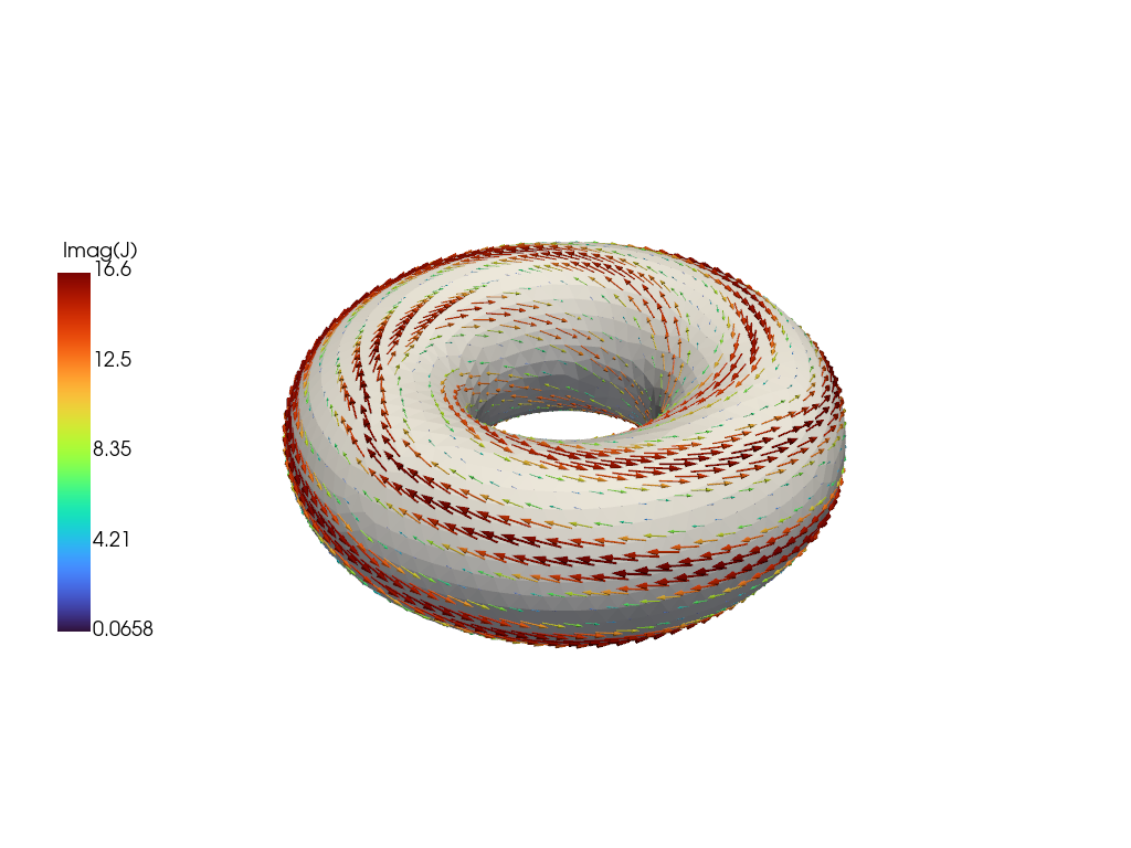
Save currents to plot files

The resulting currents are saved for plotting using tw_plate.save_current(). Here we save the real (Jr) and Imaginary (Ji) components of the response for visualization. Once all fields have been saved for plotting tw_plate.build_XDMF() to generate the XDMF descriptor files for plotting with VisIt of Paraview.

tw_coil.save_current(result[0,:],'Jr_coil')
tw_coil.save_current(result[1,:],'Ji_coil')
build_XDMF(path='.')

Removing old Xdmf files
Creating output files

Compute sensor mutual inductance matrices

We can also compute the pickup of sensors in response to both the coil and the eddy currents. To do this we compute the mutual coupling matrices between the sensors and model and the sensors and the driver coils (icoils).

Msensor, Msc, _ = tw_coil.compute_Msensor('floops.loc')

 Loading floop information:
   # of floops =           2
 Building element->sensor inductance matrix
 Building coil->sensor inductance matrix

Print probe signals for frequency response

probe_signals = np.dot(result,Msensor)
probe_signals[0,:] += np.dot(np.r_[1.E4],Msc)
for i in range(probe_signals.shape[1]):
    print('Real: {0:13.5E}, Imaginary: {1:13.5E}'.format(*probe_signals[:,i]))

Real:  -4.91207E-06, Imaginary:  -1.37454E-08
Real:   3.89336E-06, Imaginary:  -1.95259E-08

Setup plasma mode driver model

tw_mode = ThinCurr(nthreads=4)
tw_mode.setup_model(mesh_file='thincurr_mode.h5')
with h5py.File('thincurr_mode.h5', 'r+') as h5_file:
    mode_drive = np.asarray(h5_file['thincurr/driver'])

Creating thin-wall model
 Orientation depth =       12640
  Loading V(t) driver coils
  Loading I(t) driver coils

  # of points    =         6320
  # of edges     =        18960
  # of cells     =        12640
  # of holes     =            3
  # of Vcoils    =            0
  # of closures  =            2
  # of Icoils    =            0

  Building holes


WARNING: Unable to find "thincurr" XML node
WARNING: No "thincurr" XML node, using "eta=mu0" for all regions

Compute coupling from plasma mode to torus model

mode_driver = tw_mode.cross_eval(tw_coil,mode_drive)

 Applying MF element<->element inductance matrix
     Time = 24s

Compute frequency-response to plasma modes

result = tw_coil.compute_freq_response(fdriver=mode_driver,freq=1.E-3)

 Starting Frequency-response run
   Frequency [Hz] =   1.00000E-03
 Starting GMRES solver
     0  0.000000E+00  5.096814E-04
    60  1.688020E-04  9.784296E-07  5.796316E-03
   120  1.732213E-04  4.697510E-07  2.711855E-03
   180  1.852839E-04  3.538349E-07  1.909690E-03
   240  1.927548E-04  2.728285E-07  1.415417E-03
   300  2.043648E-04  2.103251E-07  1.029165E-03
   360  2.102327E-04  1.653286E-07  7.864074E-04
   420  2.190889E-04  1.267897E-07  5.787135E-04
   480  2.228605E-04  9.916932E-08  4.449839E-04
   540  2.293144E-04  7.454560E-08  3.250803E-04
   600  2.314995E-04  5.727873E-08  2.474249E-04
   660  2.359685E-04  4.181621E-08  1.772110E-04
   720  2.371472E-04  3.116136E-08  1.314009E-04
   780  2.400631E-04  2.169509E-08  9.037242E-05
   840  2.406268E-04  1.547133E-08  6.429593E-05
   900  2.423754E-04  1.004465E-08  4.144253E-05
   960  2.426093E-04  6.695185E-09  2.759657E-05
  1020  2.435300E-04  3.884133E-09  1.594930E-05
  1080  2.436085E-04  2.325438E-09  9.545798E-06
  1140  2.439946E-04  1.128253E-09  4.624091E-06
  1200  2.440139E-04  5.674469E-10  2.325470E-06
  1260  2.441252E-04  2.004905E-10  8.212610E-07
  1320  2.441277E-04  7.475196E-11  3.062002E-07
  1380  2.441441E-04  1.559556E-11  6.387851E-08
   Time =    4.4159490000000003

Compute sensor mutual inductance matrices

tw_coil.save_current(result[0,:],'Jr_mode')
tw_coil.save_current(result[1,:],'Ji_mode')
tw_coil.build_XDMF()

Removing old Xdmf files
Creating output files

Msensor_plasma, _, _ = tw_mode.compute_Msensor('floops.loc')

 Loading floop information:
   # of floops =           2
 Building element->sensor inductance matrix
 Building coil->sensor inductance matrix

Print probe signals for frequency response

probe_signals = np.dot(result,Msensor) + np.dot(mode_drive,Msensor_plasma)
for i in range(probe_signals.shape[1]):
    print('Real: {0:13.5E}, Imaginary: {1:13.5E}'.format(*probe_signals[:,i]))

Real:  -2.86249E-01, Imaginary:  -8.96706E-06
Real:  -1.22518E-01, Imaginary:   6.46085E-06

Plot current fields

Load data from plot files

with h5py.File('mesh.0001.h5','r') as h5_file:
    r = np.asarray(h5_file['R_surf'])
    lc = np.asarray(h5_file['LC_surf'])
with h5py.File('vector_dump.0001.h5','r') as h5_file:
    Ji = np.asarray(h5_file['Ji_mode_v0000'])

Create pyvista mesh for plotting

celltypes = np.array([pyvista.CellType.TRIANGLE for _ in range(lc.shape[0])], dtype=np.int8)
cells = np.insert(lc, [0,], 3, axis=1)
grid = pyvista.UnstructuredGrid(cells, celltypes, r)
grid["vectors"] = Ji
grid.set_active_vectors("vectors")

Plot current vectors on surface

p = pyvista.Plotter()
scale = 0.2/(np.linalg.norm(Ji,axis=1)).max()
arrows = grid.glyph(scale="vectors", orient="vectors", factor=scale)
p.add_mesh(arrows, cmap="turbo", scalar_bar_args={'title': "Imag(J)", "vertical": True, "position_y":0.25, "position_x": 0.05})
p.add_mesh(grid, color="white", opacity=1.0, show_edges=False)
p.show(jupyter_backend='static')