In this example we show how toroidally non-continuous conductors can be used to model different conditions in LTX-β, including:

Computing eddy currents during the OH pre-charge
Solving for an two sequential "inverse" equilibria, with self-consistent eddy currents between them
Computing vessel and plasma eigenmodes

This example utilizes the mesh built in TokaMaker Meshing Example: Building a mesh with toroidally non-continuous conductors for LTX.

Warning: Toroidally non-continuous conducting regions are still in development. Please be careful when using this feature and report any issues.

Note: Running this example requires the h5py python package, which is installable using pip or other standard methods.

import os
import sys
import time
import numpy as np
import matplotlib.pyplot as plt
import matplotlib as mpl
plt.rcParams['figure.figsize']=(6,6)
plt.rcParams['font.weight']='bold'
plt.rcParams['axes.labelweight']='bold'
plt.rcParams['lines.linewidth']=2
plt.rcParams['lines.markeredgewidth']=2
%matplotlib inline
%config InlineBackend.figure_format = "retina"

Load TokaMaker library

To load the TokaMaker python module we need to tell python where to the module is located. This can be done either through the PYTHONPATH environment variable or using within a script using sys.path.append() as below, where we look for the environement variable OFT_ROOTPATH to provide the path to where the OpenFUSIONToolkit is installed (/Applications/OFT on macOS).

For meshing we will use the gs_Domain() class to build a 2D triangular grid suitable for Grad-Shafranov equilibria. This class uses the triangle code through a python wrapper.

tokamaker_python_path = os.getenv('OFT_ROOTPATH')
if tokamaker_python_path is not None:
    sys.path.append(os.path.join(tokamaker_python_path,'python'))
from OpenFUSIONToolkit import OFT_env
from OpenFUSIONToolkit.TokaMaker import TokaMaker
from OpenFUSIONToolkit.TokaMaker.meshing import load_gs_mesh
from OpenFUSIONToolkit.TokaMaker.util import create_isoflux, create_spline_flux_fun

Setup solver

Initialize TokaMaker object

We now create a OFT_env instance for execution using two threads and a TokaMaker instance to use for equilibrium calculations. Note at present only a single TokaMaker instance can be used per python kernel, so this command should only be called once in a given Jupyter notebook or python script. In the future this restriction may be relaxed.

myOFT = OFT_env(nthreads=2)

mygs = TokaMaker(myOFT)

#----------------------------------------------
Open FUSION Toolkit Initialized
Development branch:   v1_beta6
Revision id:          681e857
Parallelization Info:
  # of MPI tasks      =    1
  # of NUMA nodes     =    1
  # of OpenMP threads =    2
Fortran input file    = /var/folders/52/n5qxh27n4w19qxzqygz2btbw0000gn/T/oft_64730/oftpyin
XML input file        = none
Integer Precisions    =    4   8
Float Precisions      =    4   8  16
Complex Precisions    =    4   8
LA backend            = native
#----------------------------------------------

Load mesh into TokaMaker

Now we load the mesh generated in TokaMaker Meshing Example: Building a mesh with toroidally non-continuous conductors for LTX using load_gs_mesh() and setup_mesh(). Then we use setup_regions() to define the different region types. Finally, we call setup() to setup the required solver objects. During this call we can specify the desired element order (min=2, max=4) and the toroidal field through F0 = B0*R0, where B0 is the toroidal field at a reference location R0.

We also increase the maximum number of Picard iterations in the equilibrium solve to 80 from the default of 40.

mesh_pts,mesh_lc,mesh_reg,coil_dict,cond_dict = load_gs_mesh('LTX_mesh.h5')
mygs.settings.maxits=80
mygs.setup_mesh(mesh_pts, mesh_lc, mesh_reg)
mygs.setup_regions(cond_dict=cond_dict,coil_dict=coil_dict)
mygs.setup(order=2, F0=0.10752)

**** Loading OFT surface mesh

**** Generating surface grid level  1
  Generating boundary domain linkage
  Mesh statistics:
    Area         =  2.640E+00
    # of points  =    3128
    # of edges   =    9241
    # of cells   =    6114
    # of boundary points =     140
    # of boundary edges  =     140
    # of boundary cells  =     140
  Resolution statistics:
    hmin =  2.294E-03
    hrms =  3.355E-02
    hmax =  7.597E-02
  Surface grounded at vertex     497


**** Creating Lagrange FE space
  Order  =    2
  Minlev =   -1

 Computing flux BC matrix 
 Inverting real matrix
   Time =    1.9570000000000000E-003

Define a vertical stability coil

Like many elongated equilibria, the equilibrium we seek to compute below is vertically unstable. In this case we use the "INTERNAL" coils in order to help with convergence using the set_coil_vsc() method, but in practice this stability is likely provided largely by the shell when plasma are sufficiently elongated.

mygs.set_coil_vsc({'INTERNALU': 1.0, 'INTERNALL': -1.0})

Define hard limits on coil currents

Hard limits on coil currents can be set using set_coil_bounds(). In this case we just the simple and approximate bi-directional limit of 50 MA in each coil.

Bounds are specified using a dictionary of 2 element lists, containing the minimum and maximum bound, where the dictionary key corresponds to the coil names, which are available in mygs.coil_sets

coil_bounds = {}
for name in mygs.coil_sets:
    if name.startswith('OH'):
        bounds = [-20.E3, 20.E3]
    elif name.startswith('RED'):
        bounds = [-5.E3, 5.E3]
    elif name.startswith('INTERNAL'):
        bounds = [-10.E3, 10.E3]
    elif name.startswith('GREEN'):
        bounds = [-2.E3, 2.E3]
    elif name.startswith('YELLOW'):
        bounds = [-50.E3, 50.E3]
    elif name.startswith('ORANGE'):
        bounds = [-10.E3, 10.E3]
    elif name.startswith('BLUE'):
        bounds = [-10.E3, 10.E3]
    coil_bounds[name] = np.array(bounds)
coil_bounds['#VSC'] = [-5.E3, 5.E3] # VS set
mygs.set_coil_bounds(coil_bounds)

Compute eddy currents during OH pre-charge

Here we demonstrate how to compute the evolution of vacuum fields in TokaMaker due to specified coil current waveforms and subject to eddy currents in conducting structures. For this example, we are using the "OH precharge", which is typical of most pulsed tokamaks, where the OH transformer is initially ramped to its maximum current (positive or negative) to allow the largest possible swing over the course of the shot ( \(\Delta I_{OH} \approx 2*I_{OH,max}\)). For this example we are ramping to the maximum current over 10 ms.

coil_currents = {key: 0.0 for key in mygs.coil_sets}
OH_curr_waveform = np.array([
    [0.0,0.0],
    [1.E-2,coil_bounds['OH'][0]],
    [1.0,coil_bounds['OH'][0]]
])

Compute Sequence of Vacuum Equilibria

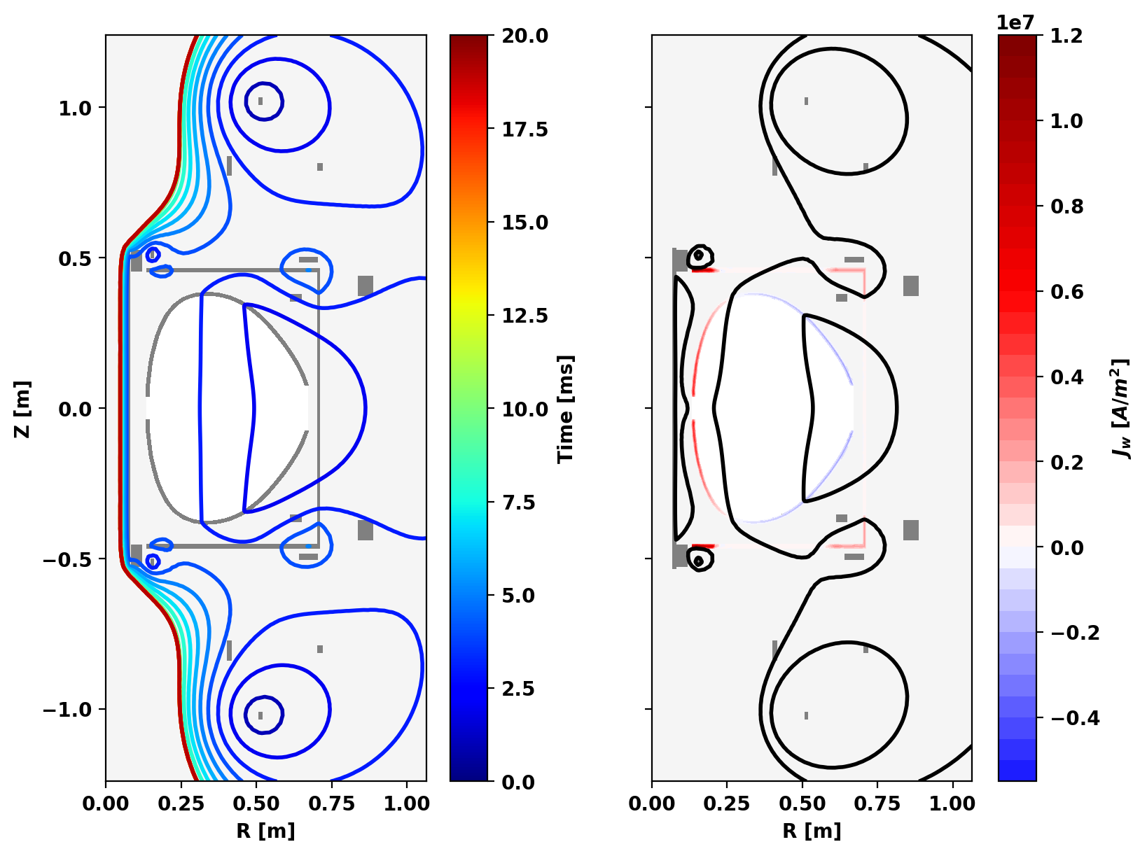
To view the evolution of the magnetic field and eddy currents during this time we compute a series of vacuum equilibria using vac_solve() from t=0 to t=20 ms. At each time point we set the coil current in the OH coil according to the waveform above and use the last state as the reference \(\psi\) for set_psi_dt().

psi_last = np.zeros((mygs.np))
t = 0.0
dt = 1.E-3
results = [psi_last]
sim_time = [0.0]
mygs.settings.pm=False
mygs.update_settings()
for i in range(20):
    t += dt
    # Update coil current
    coil_currents['OH'] = np.interp(t,OH_curr_waveform[:,0],OH_curr_waveform[:,1])
    mygs.set_coil_currents(coil_currents)
    # Solve for new state
    mygs.set_psi_dt(psi_last,dt)
    psi_new = mygs.vac_solve()
    # Save timestep for plotting
    results.append(psi_new)
    sim_time.append(t)
    # Move to previous state
    psi_last = psi_new

Plot Results

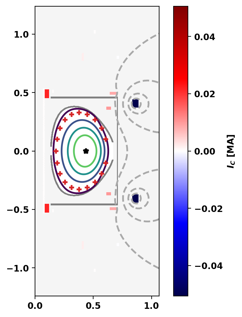
After computing the evolution of the flux we plot the motion of a given as it soaks through the conducting structures and into the bore of the OH. We also plot the eddy currents and \(\psi\) at t=10 ms to show an example distribution of eddy currents during the pre-charge.

fig, ax = plt.subplots(1,2,sharey=True,figsize=(8,6),constrained_layout=True)
# Plot flux evolution in time
mygs.plot_machine(fig,ax[0],coil_colormap=None,limiter_color=None)
colors = plt.cm.jet(np.linspace(0, 1, len(results)))
for i, result in enumerate(results[1:]):
    mygs.plot_psi(fig,ax[0],psi=-result,normalized=False,plasma_levels=[2.E-3],plasma_color=[colors[i]],vacuum_levels=None,xpoint_color=None)
norm = mpl.colors.Normalize(vmin=0.0, vmax=sim_time[-1]*1.E3)
fig.colorbar(mpl.cm.ScalarMappable(norm=norm, cmap=plt.cm.jet),ax=ax[0],label='Time [ms]')
ax[0].set_ylabel('Z [m]')
ax[0].set_xlabel('R [m]')
# Plot snapshot at t=10 ms
mygs.plot_machine(fig,ax[1],coil_colormap=None,limiter_color=None)
mygs.plot_eddy(fig,ax[1],psi=results[10],colormap='seismic',symmap=True)
mygs.plot_psi(fig,ax[1],psi=-results[10],normalized=False,plasma_levels=[4.7E-3,6.E-3],plasma_color='k',vacuum_levels=None,xpoint_color=None)
_ = ax[-1].set_xlabel('R [m]')

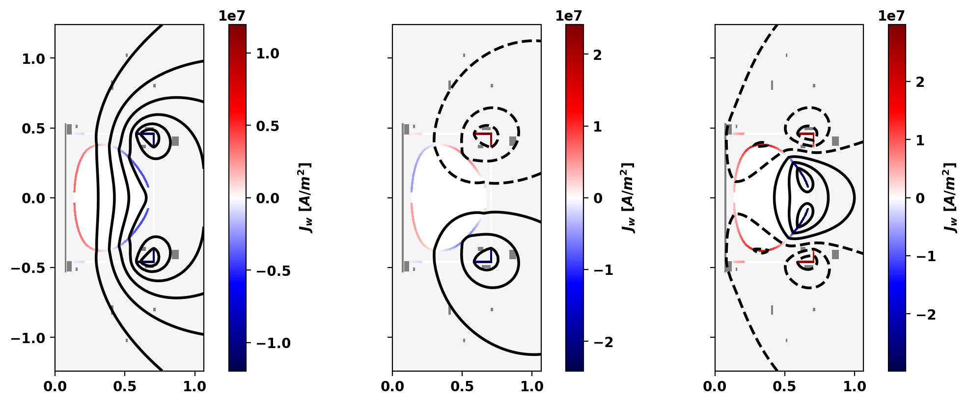
Compute Decay Modes of Conductor System

Here we compute the decay modes (L/R eigenvalues) of the conductors in our model.

psi0 = mygs.get_psi(False)
eig_vals, eig_vecs = mygs.eig_wall(10)
fig, ax = plt.subplots(1,3,sharey=True,figsize=(10,4),constrained_layout=True)
for i in range(3):
    mygs.plot_machine(fig,ax[i],limiter_color=None)
    mygs.plot_psi(fig,ax[i],eig_vecs[i,:],xpoint_color=None,opoint_color=None,normalized=False,plasma_color='k')
    mygs.plot_eddy(fig,ax[i],dpsi_dt=eig_vecs[i,:]*abs(eig_vals[i,0]),colormap='seismic',symmap=True)
print('Longest L/R time = {0:.4E} [s]'.format(1.0/eig_vals[0,0]))

Longest L/R time = 5.1203E-03 [s]

Compute flattop-like equilibrium

Define global quantities and targets

For the inverse case we define a target for the plasma current and the ratio the F*F' and P' contributions to the plasma current, which is approximately related to \(\beta_p\) as Ip_ratio = \(1/\beta_p - 1\).

Note: These constraints can be considered "hard" constraints, where they will be matched to good tolerance as long as the calculation converges.

Ip_target = 8.0E4

mygs.set_targets(Ip=Ip_target,Ip_ratio=2.0)

Define shape targets

In order to constrain the shape of the plasma we can utilize isoflux points, which are points we want to lie on the same flux surface (eg. the LCFS).

Note: These constraints can be considered "soft" constraints, where the calculation attempts to minimize error in satisfying these constraints subject to other constraints and regularization.

Here we define a somewhat large number of isoflux points that we want to lie on a single surface of the target equilibrium.

isoflux_pts = create_isoflux(20,0.40,0.0,0.22,1.5,0.1)

mygs.set_isoflux(isoflux_pts)

Define coil regularization matrix

In general, for a given coil set a given plasma shape cannot be exactly reproduced, which generally yields large amplitude coil currents if no constraint on the coil currents is applied. As a result, it is useful to include regularization terms for the coils to balance minimization of the shape error with the amplitude of current in the coils. In TokaMaker these regularization terms have the general form, where each term corresponds to a set of coil coefficients, target value, and weight. The coil_reg_term() method is provided to aid in defining these terms.

Here we define two types of regularization targets:

Targets that act to penalize up-down assymetry in U/L coil pairs
Targets the act to penalize the amplitude of current in each coil

In the later case this regularization acts to penalize the amplitude of current in each coil, acting to balance coil current with error in the shape targets. Additionally, this target is also used to "disable" the YELLOW coil by setting the weight on its target high to strongly penalize non-zero current.

disable_list = ('YELLOW',)
 
# Set regularization weights
regularization_terms = []
for name, coil in mygs.coil_sets.items():
    if name[:-1] in disable_list:
        # Set zero target current and high weight on coil
        regularization_terms.append(mygs.coil_reg_term({name: 1.0},target=0.0,weight=1.E4))
        continue
    if name == 'OH': # OH coil has no mirror
        # Set zero target current and small weight to help conditioning of fit
        regularization_terms.append(mygs.coil_reg_term({name: 1.0},target=0.0,weight=1.E-1))
        continue
    elif name[-1] == 'L':
        continue
    # Set zero target current and small weight to help conditioning of fit
    regularization_terms.append(mygs.coil_reg_term({name: 1.0},target=0.0,weight=1.E-1))
    # Set zero target for the difference of currents for coil and its mirror to ensure up-down symmetry
    regularization_terms.append(mygs.coil_reg_term({name: 1.0, name[:-1]+'L': -1.0},target=0.0,weight=1.E2))
# Set zero target current and small weight on virtual VSC to allow up-down adjustment
regularization_terms.append(mygs.coil_reg_term({'#VSC': 1.0},target=0.0,weight=1.E-4))
 
# Pass regularization terms to TokaMaker
mygs.set_coil_reg(reg_terms=regularization_terms)

Define flux functions

Although TokaMaker has a "default" profile for the F*F' and P' terms this should almost never be used and one should instead choose an appropriate flux function for their application. In this case we use a simple cubic flux function, using create_spline_flux_fun(), with the same shape for both F*F' and P'. Within TokaMaker this profile is represented as a piecewise linear function, which can be set up using the dictionary approach shown below.

prof = create_spline_flux_fun(40,[0.0,0.5,1.0],[1.0,0.5,0.0],axis_bc=[1,0.0],edge_bc=[1,0.0])
plt.plot(prof['x'],prof['y'])
mygs.set_profiles(ffp_prof=prof,pp_prof=prof)

Compute initial equilibrium

We can now compute a free-boundary equilibrium using these constraints. Note that before running a calculation for the first time we must initialize the flux function \(\psi\), which can be done using init_psi. This subroutine initializes the flux using the specified Ip_target from above, which is evenly distributed over the entire plasma region or only with a boundary defined using a center point (R,Z), minor radius (a), and elongation and triangularity. Coil currents are also initialized at this point using the constraints above and this uniform plasma current initialization.

We plot the solution and coil currents after initialization but before the Grad-Shafranov solve for reference.

solve is then called to compute a self-consitent Grad-Shafranov equilibrium. If the result variable (err_flag) is zero then the solution has converged to the desired tolerance ( \(10^{-6}\) by default).

# Disable eddy currents by removing reference state (dt < 0)
dt=1.0
mygs.set_psi_dt(0.0*mygs.get_psi(False),-dt)
# Initialize solve with a simple current shape
mygs.init_psi(0.42,0.0,0.15,1.5,0.6)
# Re-enable iteration output
mygs.settings.pm=True
mygs.update_settings()
# Compute equilbrium and save flux for later
mygs.solve()
psi_last = mygs.get_psi(False)

Starting non-linear GS solver
     1  4.1858E-01  6.6300E-01  2.7602E-03  4.3541E-01  8.6918E-05 -4.1733E-01
     2  4.8533E-01  7.5420E-01  1.0732E-03  4.3544E-01  8.2293E-05 -2.9882E-01
     3  5.1712E-01  7.9707E-01  4.4141E-04  4.3567E-01  7.6874E-05 -2.9624E-01
     4  5.3378E-01  8.1932E-01  2.0386E-04  4.3589E-01  7.3108E-05 -2.8162E-01
     5  5.4279E-01  8.3126E-01  1.0251E-04  4.3604E-01  7.1115E-05 -2.6197E-01
     6  5.4772E-01  8.3776E-01  5.4047E-05  4.3613E-01  7.0010E-05 -2.4857E-01
     7  5.5044E-01  8.4132E-01  2.9203E-05  4.3619E-01  6.9297E-05 -2.4431E-01
     8  5.5194E-01  8.4328E-01  1.5971E-05  4.3623E-01  6.8838E-05 -2.4409E-01
     9  5.5277E-01  8.4437E-01  8.7860E-06  4.3625E-01  6.8557E-05 -2.4332E-01
    10  5.5323E-01  8.4496E-01  4.8495E-06  4.3626E-01  6.8391E-05 -2.4281E-01
    11  5.5348E-01  8.4530E-01  2.6817E-06  4.3627E-01  6.8296E-05 -2.4248E-01
    12  5.5363E-01  8.4548E-01  1.4846E-06  4.3627E-01  6.8240E-05 -2.4218E-01
    13  5.5371E-01  8.4558E-01  8.2246E-07  4.3627E-01  6.8207E-05 -2.4195E-01
 Timing:   8.3265999972354621E-002
   Source:     3.4822000132407993E-002
   Solve:      2.2271999972872436E-002
   Boundary:   2.1390000474639237E-003
   Other:      2.4032999819610268E-002

Plot equilibrium

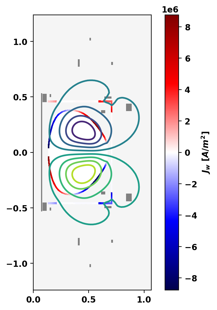
Flux surfaces of the computed equilibrium can be plotted using the plot_psi() method. The additional plotting methods plot_machine() and plot_constraints() are also used to show context and other information. Each method has a large number of optional arguments for formatting and other options. We also use plot_eddy() to show the eddy currents in the vessel due to the change in flux from the preceding equilibrium.

Basic parameters can be displayed using the print_info() method. For access to these quantities as variables instead the get_stats() can be used.

The final coil currents can also be retrieved using the get_coil_currents() method, which are all within the approximate coil limits imposed above.

# Plot equilibrium
fig, ax = plt.subplots(1,1)
mygs.plot_machine(fig,ax,coil_colormap='seismic',coil_scale=1.E-6,coil_clabel=r'$I_C$ [MA]',coil_symmap=True,limiter_color=None)
mygs.plot_psi(fig,ax,plasma_nlevels=5,vacuum_nlevels=5)
mygs.plot_constraints(fig, ax)
# Print information and coil currents
mygs.print_info()
print()
print("Coil Currents [kA]:")
coil_currents, _ = mygs.get_coil_currents()
for key in coil_currents:
    if coil_currents[key] >= 0.0:
        proximity = coil_currents[key]*100/coil_bounds[key][1]
        near_limit = coil_bounds[key][1]
    else:
        proximity = coil_currents[key]*100/coil_bounds[key][0]
        near_limit = coil_bounds[key][0]
    print('  {0:10} {1:10.2F} ({2:7.2F}) [{3:6.2F}%]'.format(key+":",coil_currents[key]/1.E3,near_limit/1.E3,proximity))

Equilibrium Statistics:
  Topology                =   Limited
  Toroidal Current [A]    =    7.9994E+04
  Current Centroid [m]    =    0.407  0.000
  Magnetic Axis [m]       =    0.436  0.000
  Elongation              =    1.537 (U:  1.537, L:  1.537)
  Triangularity           =    0.130 (U:  0.129, L:  0.131)
  Plasma Volume [m^3]     =    0.643
  q_0, q_95               =    1.266  6.309
  Plasma Pressure [Pa]    =   Axis:  1.7620E+03, Peak:  1.7620E+03
  Stored Energy [J]       =    3.7342E+02
  <Beta_pol> [%]          =   34.6606
  <Beta_tor> [%]          =    1.3011
  <Beta_n>   [%]          =    1.0473
  Diamagnetic flux [Wb]   =    8.6550E-04
  Toroidal flux [Wb]      =    8.3542E-02
  l_i                     =    1.1889

Coil Currents [kA]:
  REDU:            0.70 (   5.00) [ 13.94%]
  REDL:            0.70 (   5.00) [ 13.94%]
  ORANGEU:         0.09 (  10.00) [  0.93%]
  ORANGEL:         0.09 (  10.00) [  0.93%]
  YELLOWU:        -0.00 ( -50.00) [  0.00%]
  YELLOWL:        -0.00 ( -50.00) [  0.00%]
  GREENU:          0.43 (   2.00) [ 21.49%]
  GREENL:          0.43 (   2.00) [ 21.49%]
  BLUEU:          -4.22 ( -10.00) [ 42.17%]
  BLUEL:          -4.22 ( -10.00) [ 42.17%]
  INTERNALU:       2.00 (  10.00) [ 19.99%]
  INTERNALL:       2.00 (  10.00) [ 20.00%]
  OH:              0.00 (  20.00) [  0.02%]

Compute equilibrium 5 ms later

# Set prior flux state
mygs.set_psi_dt(psi_last,5.E-3)
# Update Ip target
Ip_target = 9.0E4
mygs.set_targets(Ip=Ip_target,Ip_ratio=2.0)
# Compute new equilbrium and save flux for later
mygs.solve()
psi_new = mygs.get_psi(False)

Starting non-linear GS solver
     1  6.2297E-01  9.5134E-01  4.1997E-04  4.3736E-01  5.7378E-05 -2.7201E-01
     2  6.3261E-01  9.5593E-01  2.0964E-04  4.3754E-01  5.5415E-05 -3.0402E-01
     3  6.3255E-01  9.5654E-01  7.5082E-05  4.3733E-01  5.7456E-05 -2.9697E-01
     4  6.2977E-01  9.5518E-01  3.6082E-05  4.3703E-01  6.0377E-05 -2.7628E-01
     5  6.2682E-01  9.5329E-01  3.1462E-05  4.3678E-01  6.2947E-05 -2.6750E-01
     6  6.2456E-01  9.5163E-01  2.5292E-05  4.3660E-01  6.4777E-05 -2.6652E-01
     7  6.2306E-01  9.5042E-01  1.7683E-05  4.3649E-01  6.5944E-05 -2.6756E-01
     8  6.2215E-01  9.4964E-01  1.1181E-05  4.3643E-01  6.6620E-05 -2.6859E-01
     9  6.2165E-01  9.4916E-01  6.5567E-06  4.3639E-01  6.6980E-05 -2.6950E-01
    10  6.2138E-01  9.4889E-01  3.6173E-06  4.3638E-01  6.7157E-05 -2.7017E-01
    11  6.2125E-01  9.4874E-01  1.8940E-06  4.3637E-01  6.7238E-05 -2.7058E-01
    12  6.2119E-01  9.4867E-01  9.4699E-07  4.3637E-01  6.7271E-05 -2.7081E-01
 Timing:  0.15450499998405576     
   Source:     3.2104999991133809E-002
   Solve:      1.9957999989856035E-002
   Boundary:   2.2590000298805535E-003
   Other:     0.10018299997318536

Plot equilibrium

We now show the updated equilibrium, this time using plot_eddy() to show the eddy currents in the vessel due to the change in flux from the preceding equilibrium.

# Plot equilibrium
fig, ax = plt.subplots(1,1)
mygs.plot_machine(fig,ax,limiter_color=None)
mygs.plot_psi(fig,ax,plasma_nlevels=5,vacuum_nlevels=5)
mygs.plot_eddy(fig,ax,psi=psi_new,colormap='seismic',symmap=True)
mygs.plot_constraints(fig, ax)
# Print information and coil currents
mygs.print_info()
print()
print("Coil Currents [kA]:")
coil_currents, _ = mygs.get_coil_currents()
for key in coil_currents:
    if coil_currents[key] >= 0.0:
        proximity = coil_currents[key]*100/coil_bounds[key][1]
        near_limit = coil_bounds[key][1]
    else:
        proximity = coil_currents[key]*100/coil_bounds[key][0]
        near_limit = coil_bounds[key][0]
    print('  {0:10} {1:10.2F} ({2:7.2F}) [{3:6.2F}%]'.format(key+":",coil_currents[key]/1.E3,near_limit/1.E3,proximity))

Starting CG solver
     0  0.000000E+00  0.000000E+00  2.570366E-02
     1 -2.919869E+00  2.672399E+02  9.998829E-03  3.741518E-05
     2 -3.393750E+00  3.019796E+02  4.391137E-03  1.454117E-05
     3 -3.454844E+00  3.104265E+02  1.630672E-03  5.253004E-06
     4 -3.463806E+00  3.107788E+02  6.490879E-04  2.088585E-06
     5 -3.465284E+00  3.100384E+02  2.386736E-04  7.698197E-07
     6 -3.465484E+00  3.094506E+02  8.786765E-05  2.839473E-07
     7 -3.465516E+00  3.093363E+02  3.700683E-05  1.196330E-07
     8 -3.465520E+00  3.093555E+02  1.637065E-05  5.291856E-08
     9 -3.465521E+00  3.093739E+02  6.449134E-06  2.084576E-08
    10 -3.465521E+00  3.093818E+02  2.274598E-06  7.352074E-09
    20 -3.465521E+00  3.093829E+02  1.742395E-10  5.631839E-13
Equilibrium Statistics:
  Topology                =   Limited
  Toroidal Current [A]    =    9.0004E+04
  Current Centroid [m]    =    0.407  0.000
  Magnetic Axis [m]       =    0.436  0.000
  Elongation              =    1.538 (U:  1.538, L:  1.538)
  Triangularity           =    0.133 (U:  0.135, L:  0.132)
  Plasma Volume [m^3]     =    0.644
  q_0, q_95               =    1.143  5.644
  Plasma Pressure [Pa]    =   Axis:  2.2242E+03, Peak:  2.2242E+03
  Stored Energy [J]       =    4.7273E+02
  <Beta_pol> [%]          =   34.7576
  <Beta_tor> [%]          =    1.6411
  <Beta_n>   [%]          =    1.1767
  Diamagnetic flux [Wb]   =    1.0908E-03
  Toroidal flux [Wb]      =    8.4048E-02
  l_i                     =    1.1911

Coil Currents [kA]:
  REDU:            0.74 (   5.00) [ 14.74%]
  REDL:            0.74 (   5.00) [ 14.74%]
  ORANGEU:         0.14 (  10.00) [  1.38%]
  ORANGEL:         0.14 (  10.00) [  1.38%]
  YELLOWU:        -0.00 ( -50.00) [  0.00%]
  YELLOWL:        -0.00 ( -50.00) [  0.00%]
  GREENU:          0.50 (   2.00) [ 25.02%]
  GREENL:          0.50 (   2.00) [ 25.02%]
  BLUEU:          -4.83 ( -10.00) [ 48.30%]
  BLUEL:          -4.83 ( -10.00) [ 48.30%]
  INTERNALU:       2.16 (  10.00) [ 21.58%]
  INTERNALL:       2.16 (  10.00) [ 21.59%]
  OH:              0.00 (  20.00) [  0.01%]

Linear Stability Analysis

We can compute the most unstable eigenmodes of the linearized system along with their eigenvalues, or growth rates, using the eig_td() method. In this case, the most unstable mode corresponds to vertical instability, and has a growth rate of ~480 s^-1.

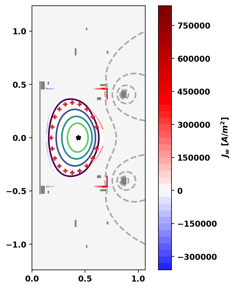
We also plot the vertically unstable mode and the eddy currents in conducting structures using the plot_eddy() method.

psi0 = mygs.get_psi(False)
eig_vals, eig_vecs = mygs.eig_td(-2.E4,10,False)
fig, ax = plt.subplots(1,1)
mygs.plot_machine(fig,ax,limiter_color=None)
mygs.plot_psi(fig,ax,eig_vecs[0,:],xpoint_color=None,opoint_color=None,normalized=False,plasma_nlevels=10)
mygs.plot_eddy(fig,ax,dpsi_dt=eig_vecs[0,:]*abs(eig_vals[0,0]),colormap='seismic')
print('Growth rate = {0:.2F} [1/s]'.format(eig_vals[0,0]))

Growth rate = -481.12 [1/s]