In this example we show how to compute eddy currents and resulting forces from a simplified disruptive current quench in ITER.
This example utilizes the mesh built in TokaMaker Meshing Example: Building a mesh for ITER.
- Note
- Running this example requires the h5py python package, which is installable using
pip or other standard methods.
import os
import sys
import numpy as np
import matplotlib.pyplot as plt
import matplotlib as mpl
plt.rcParams['figure.figsize']=(6,6)
plt.rcParams['font.weight']='bold'
plt.rcParams['axes.labelweight']='bold'
plt.rcParams['lines.linewidth']=2
plt.rcParams['lines.markeredgewidth']=2
%matplotlib inline
%config InlineBackend.figure_format = "retina"
Load TokaMaker library
To load the TokaMaker python module we need to tell python where to the module is located. This can be done either through the PYTHONPATH environment variable or using within a script using sys.path.append() as below, where we look for the environement variable OFT_ROOTPATH to provide the path to where the OpenFUSIONToolkit is installed (/Applications/OFT on macOS).
For meshing we will use the gs_Domain class to build a 2D triangular grid suitable for Grad-Shafranov equilibria. This class uses the triangle code through a python wrapper.
tokamaker_python_path = os.getenv('OFT_ROOTPATH')
if tokamaker_python_path is not None:
sys.path.append(os.path.join(tokamaker_python_path,'python'))
from OpenFUSIONToolkit import OFT_env
Compute pre-CQ equilibrium
Now we compute the same equilibrium as in TokaMaker Example: Baseline L-mode scenario in ITER.
myOFT = OFT_env(nthreads=2)
mygs = TokaMaker(myOFT)
mesh_pts,mesh_lc,mesh_reg,coil_dict,cond_dict = load_gs_mesh('ITER_mesh.h5')
mygs.setup_mesh(mesh_pts, mesh_lc, mesh_reg)
mygs.setup_regions(cond_dict=cond_dict,coil_dict=coil_dict)
mygs.setup(order = 2, F0 = 5.3*6.2)
mygs.set_coil_vsc({'VS': 1.0})
coil_bounds = {key: [-50.E6, 50.E6] for key in mygs.coil_sets}
mygs.set_coil_bounds(coil_bounds)
Ip_target=15.6E6
P0_target=6.2E5
mygs.set_targets(Ip=Ip_target, pax=P0_target)
isoflux_pts = np.array([
[ 8.20, 0.41],
[ 8.06, 1.46],
[ 7.51, 2.62],
[ 6.14, 3.78],
[ 4.51, 3.02],
[ 4.26, 1.33],
[ 4.28, 0.08],
[ 4.49, -1.34],
[ 7.28, -1.89],
[ 8.00, -0.68]
])
x_point = np.array([[5.125, -3.4],])
mygs.set_isoflux(np.vstack((isoflux_pts,x_point)))
mygs.set_saddles(x_point)
regularization_terms = []
for name, coil in mygs.coil_sets.items():
if name.startswith('CS'):
if name.startswith('CS1'):
regularization_terms.append(mygs.coil_reg_term({name: 1.0},target=0.0,weight=2.E-2))
else:
regularization_terms.append(mygs.coil_reg_term({name: 1.0},target=0.0,weight=1.E-2))
elif name.startswith('PF'):
regularization_terms.append(mygs.coil_reg_term({name: 1.0},target=0.0,weight=1.E-2))
elif name.startswith('VS'):
regularization_terms.append(mygs.coil_reg_term({name: 1.0},target=0.0,weight=1.E-2))
regularization_terms.append(mygs.coil_reg_term({'#VSC': 1.0},target=0.0,weight=1.E2))
mygs.set_coil_reg(reg_terms=regularization_terms)
ffp_prof = create_power_flux_fun(40,1.5,2.0)
pp_prof = create_power_flux_fun(40,4.0,1.0)
mygs.set_profiles(ffp_prof=ffp_prof,pp_prof=pp_prof)
R0 = 6.3
Z0 = 0.5
a = 2.0
kappa = 1.4
delta = 0.0
mygs.init_psi(R0, Z0, a, kappa, delta)
mygs.solve()
psi_full = mygs.get_psi(normalized=False)
psi_lim = mygs.psi_bounds[0]
#----------------------------------------------
Open FUSION Toolkit Initialized
Development branch:   v1_beta6
Revision id:          681e857
Parallelization Info:
  # of MPI tasks      =    1
  # of NUMA nodes     =    1
  # of OpenMP threads =    2
Fortran input file    = /var/folders/52/n5qxh27n4w19qxzqygz2btbw0000gn/T/oft_64685/oftpyin
XML input file        = none
Integer Precisions    =    4   8
Float Precisions      =    4   8  16
Complex Precisions    =    4   8
LA backend            = native
#----------------------------------------------


**** Loading OFT surface mesh

**** Generating surface grid level  1
  Generating boundary domain linkage
  Mesh statistics:
    Area         =  2.859E+02
    # of points  =    4757
    # of edges   =   14156
    # of cells   =    9400
    # of boundary points =     112
    # of boundary edges  =     112
    # of boundary cells  =     112
  Resolution statistics:
    hmin =  9.924E-03
    hrms =  2.826E-01
    hmax =  8.466E-01
  Surface grounded at vertex     870


**** Creating Lagrange FE space
  Order  =    2
  Minlev =   -1

 Computing flux BC matrix
 Inverting real matrix
   Time =    1.1280000000000001E-003
Starting non-linear GS solver
     1  5.7965E+00  1.5693E-01  6.4686E-01  6.4422E+00  5.3430E-01  9.8316E-04
     2  1.5480E+01  9.5055E-02  2.7469E-01  6.4072E+00  5.3290E-01  1.5938E-03
     3  1.9148E+01  7.9379E-02  1.2986E-01  6.3868E+00  5.3264E-01  1.6630E-03
     4  2.0951E+01  7.3407E-02  6.7604E-02  6.3757E+00  5.3235E-01  1.6305E-03
     5  2.1908E+01  7.0680E-02  3.6983E-02  6.3697E+00  5.3227E-01  1.5882E-03
     6  2.2433E+01  6.9312E-02  2.0669E-02  6.3664E+00  5.3231E-01  1.5557E-03
     7  2.2724E+01  6.8590E-02  1.1653E-02  6.3646E+00  5.3240E-01  1.5342E-03
     8  2.2888E+01  6.8198E-02  6.5944E-03  6.3636E+00  5.3250E-01  1.5207E-03
     9  2.2980E+01  6.7980E-02  3.7379E-03  6.3631E+00  5.3258E-01  1.5126E-03
    10  2.3032E+01  6.7859E-02  2.1210E-03  6.3628E+00  5.3265E-01  1.5079E-03
    11  2.3061E+01  6.7791E-02  1.2045E-03  6.3626E+00  5.3270E-01  1.5051E-03
    12  2.3078E+01  6.7753E-02  6.8471E-04  6.3625E+00  5.3274E-01  1.5035E-03
    13  2.3087E+01  6.7731E-02  3.8962E-04  6.3625E+00  5.3277E-01  1.5025E-03
    14  2.3093E+01  6.7719E-02  2.2195E-04  6.3624E+00  5.3279E-01  1.5020E-03
    15  2.3096E+01  6.7712E-02  1.2660E-04  6.3624E+00  5.3280E-01  1.5017E-03
    16  2.3097E+01  6.7708E-02  7.2329E-05  6.3624E+00  5.3281E-01  1.5015E-03
    17  2.3098E+01  6.7705E-02  4.1395E-05  6.3624E+00  5.3281E-01  1.5014E-03
    18  2.3099E+01  6.7704E-02  2.3741E-05  6.3624E+00  5.3282E-01  1.5013E-03
    19  2.3099E+01  6.7703E-02  1.3650E-05  6.3624E+00  5.3282E-01  1.5013E-03
    20  2.3099E+01  6.7703E-02  7.8710E-06  6.3624E+00  5.3282E-01  1.5013E-03
    21  2.3100E+01  6.7703E-02  4.5542E-06  6.3624E+00  5.3282E-01  1.5013E-03
    22  2.3100E+01  6.7702E-02  2.6456E-06  6.3624E+00  5.3283E-01  1.5013E-03
    23  2.3100E+01  6.7702E-02  1.5440E-06  6.3624E+00  5.3283E-01  1.5013E-03
    24  2.3100E+01  6.7702E-02  9.0578E-07  6.3624E+00  5.3283E-01  1.5013E-03
 Timing:  0.20504199998686090
   Source:     9.0769000002183020E-002
   Solve:      6.2658999871928245E-002
   Boundary:   5.4510000627487898E-003
   Other:      4.6163000050000846E-002
Print information and plot equilibrium
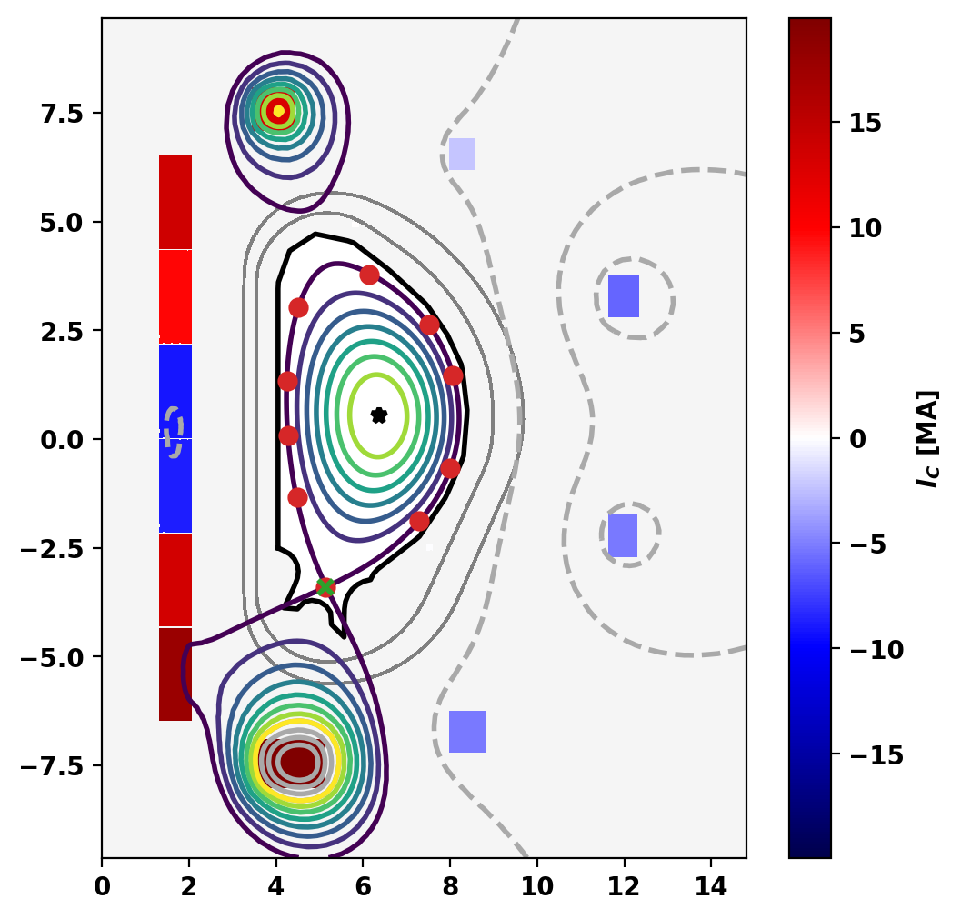
Flux surfaces of the computed equilibrium can be plotted using the plot_psi() method. The additional plotting methods plot_machine() and plot_constraints() are also used to show context and other information. Each method has a large number of optional arguments for formatting and other options.
fig, ax = plt.subplots(1,1)
mygs.plot_machine(fig,ax,coil_colormap='seismic',coil_symmap=True,coil_scale=1.E-6,coil_clabel=r'$I_C$ [MA]')
mygs.plot_psi(fig,ax,xpoint_color=None,vacuum_nlevels=4)
mygs.plot_constraints(fig,ax,isoflux_color='tab:red',isoflux_marker='o')
mygs.print_info()
print()
print("Coil Currents [MA]:")
coil_currents, _ = mygs.get_coil_currents()
for key, current in coil_currents.items():
print(' {0:10} {1:10.2F}'.format(key+":",current/1.E6))
Equilibrium Statistics:
  Topology                =   Diverted
  Toroidal Current [A]    =    1.5600E+07
  Current Centroid [m]    =    6.203  0.530
  Magnetic Axis [m]       =    6.362  0.533
  Elongation              =    1.875 (U:  1.763, L:  1.987)
  Triangularity           =    0.477 (U:  0.405, L:  0.550)
  Plasma Volume [m^3]     =   820.079
  q_0, q_95               =    0.823  2.760
  Plasma Pressure [Pa]    =   Axis:  6.1923E+05, Peak:  6.1923E+05
  Stored Energy [J]       =    2.4299E+08
  <Beta_pol> [%]          =   42.6829
  <Beta_tor> [%]          =    1.7801
  <Beta_n>   [%]          =    1.1953
  Diamagnetic flux [Wb]   =    1.5403E+00
  Toroidal flux [Wb]      =    1.2187E+02
  l_i                     =    1.1597

Coil Currents [MA]:
  CS3U:           13.74
  CS2U:            9.74
  CS1U:           -9.06
  CS1L:           -8.81
  CS2L:           13.40
  CS3L:           17.88
  PF1:            12.94
  PF2:            -2.20
  PF3:            -5.95
  PF4:            -5.14
  PF5:            -5.18
  PF6:            19.93
  VS:              0.15
Compute eddy currents and forces for a simple current quench
TokaMaker can be used to evaluate some of the impacts caused by the Current Quench (CQ) that occurs following a disruption in tokamaks. During the CQ the plasma current rapidly falls due to high resistivity following the thermal quench. In real CQs the plasma current profile significantly evolves during this quench, due to changes in pressure and temperature profiles and plasma motions, such as VDEs. However, for first order approximation we can model the eddy currents and voltages produced by the CQ by simply decreasing the flux corresponding to the plasma current over a given timescale.
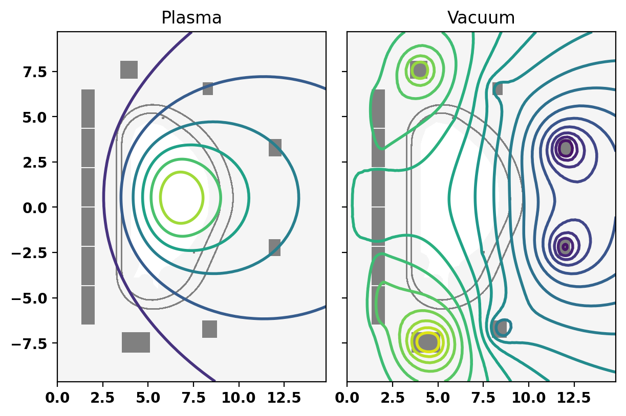
Extract flux from plasma current only
To do this we first need to separate the flux corresponding to the plasma current, which changes during the CQ, from the vacuum flux produced by the coils, which does not change (if the coil currents remain fixed) over the CQ. This can be done by performing a vacuum solve (vac_solve()) to get the vacuum flux from the coils and then subtracting this from the full flux to isolate the plasma contribution.
- Note
- This is meant to act as a first order model of inductive CQ impacts and additional effects related to the detailed evolution of the plasma current, coil currents, and other dynamics will be important for detailed analysis and/or predicitons.
mygs.set_psi(0.0*psi_full)
psi_vac = mygs.vac_solve()
psi_plasma = psi_full-psi_vac
coil_currents, _ = mygs.get_coil_currents()
fig, ax = plt.subplots(1,2,sharey=True,constrained_layout=True)
mygs.plot_machine(fig,ax[0],limiter_color=None)
mygs.plot_psi(fig,ax[0],psi_plasma,normalized=False,xpoint_color=None,opoint_color=None)
ax[0].set_title('Plasma')
mygs.plot_machine(fig,ax[1],coil_colormap=None,limiter_color=None)
mygs.plot_psi(fig,ax[1],psi=psi_vac,normalized=False,plasma_nlevels=20,vacuum_levels=None,xpoint_color=None,opoint_color=None)
_ = ax[1].set_title('Vacuum')
1 4.2217E+06
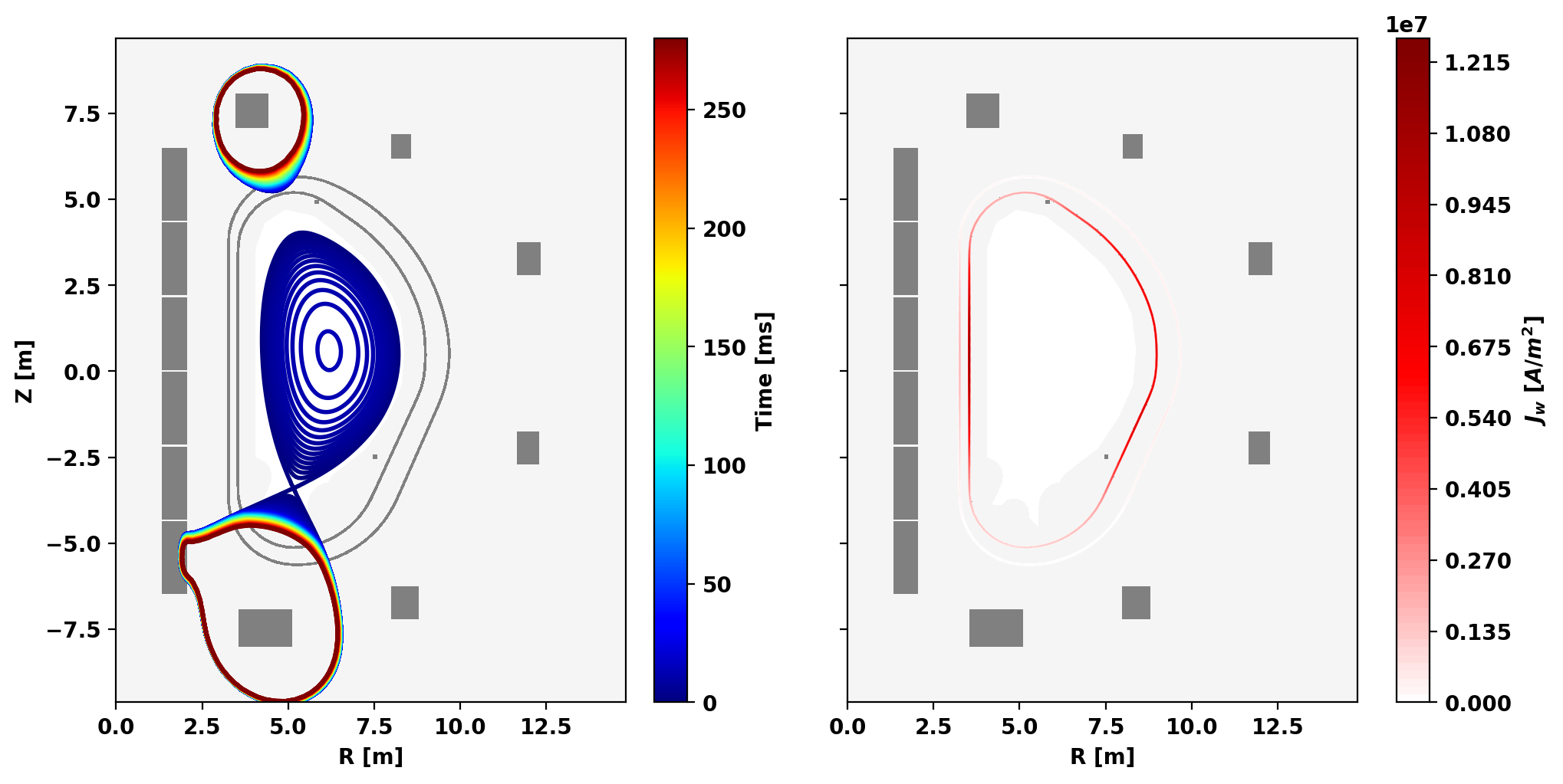
Perform time-dependent simulation with plasma-current quench source
With the flux separated into constituent components a time-dependent simulation may now be performed to compute the evolution of eddy current in conducting structures in response to the loop voltage generated by the CQ.
CQ_time = 20.0E-3
psi_last = np.zeros((mygs.np))
t = 0.0
dt = CQ_time/20.0
results = [psi_vac+psi_plasma]
sim_time = [0.0]
mygs.settings.pm=False
mygs.update_settings()
mygs.set_coil_currents()
for i in range(100):
if i == 40:
dt = CQ_time/5.0
if t <= CQ_time:
mygs.set_psi_dt(psi_plasma*dt/CQ_time+psi_last,dt)
else:
mygs.set_psi_dt(psi_last,dt)
mygs.set_psi(0.0*psi_last)
psi_last = mygs.vac_solve()
t += dt
results.append(psi_vac+psi_last+psi_plasma*max(0.0,1.0-t/CQ_time))
sim_time.append(t)
sim_time = np.array(sim_time)
ind_sample = (abs(sim_time-CQ_time/2.0)).argmin()
ind_sample2 = (abs(sim_time-CQ_time*2.0)).argmin()
Plot results
fig, ax = plt.subplots(1,2,sharey=True,figsize=(10,5),constrained_layout=True)
mygs.plot_machine(fig,ax[0],coil_colormap=None,limiter_color=None)
colors = plt.cm.jet(sim_time/sim_time[-1])
for i, result in enumerate(results):
mygs.plot_psi(fig,ax[0],psi=result,normalized=False,plasma_levels=[psi_lim],plasma_color=[colors[i]],vacuum_levels=None,xpoint_color=None,opoint_color=None)
norm = mpl.colors.Normalize(vmin=0.0, vmax=sim_time[-1]*1.E3)
fig.colorbar(mpl.cm.ScalarMappable(norm=norm, cmap=plt.cm.jet),ax=ax[0],label='Time [ms]')
mygs.plot_machine(fig,ax[1],coil_colormap=None,limiter_color=None)
mygs.plot_eddy(fig,ax[1],psi=results[ind_sample],colormap='seismic',symmap=True,nlevels=100)
ax[0].set_ylabel('Z [m]')
ax[0].set_xlabel('R [m]')
_ = ax[-1].set_xlabel('R [m]')
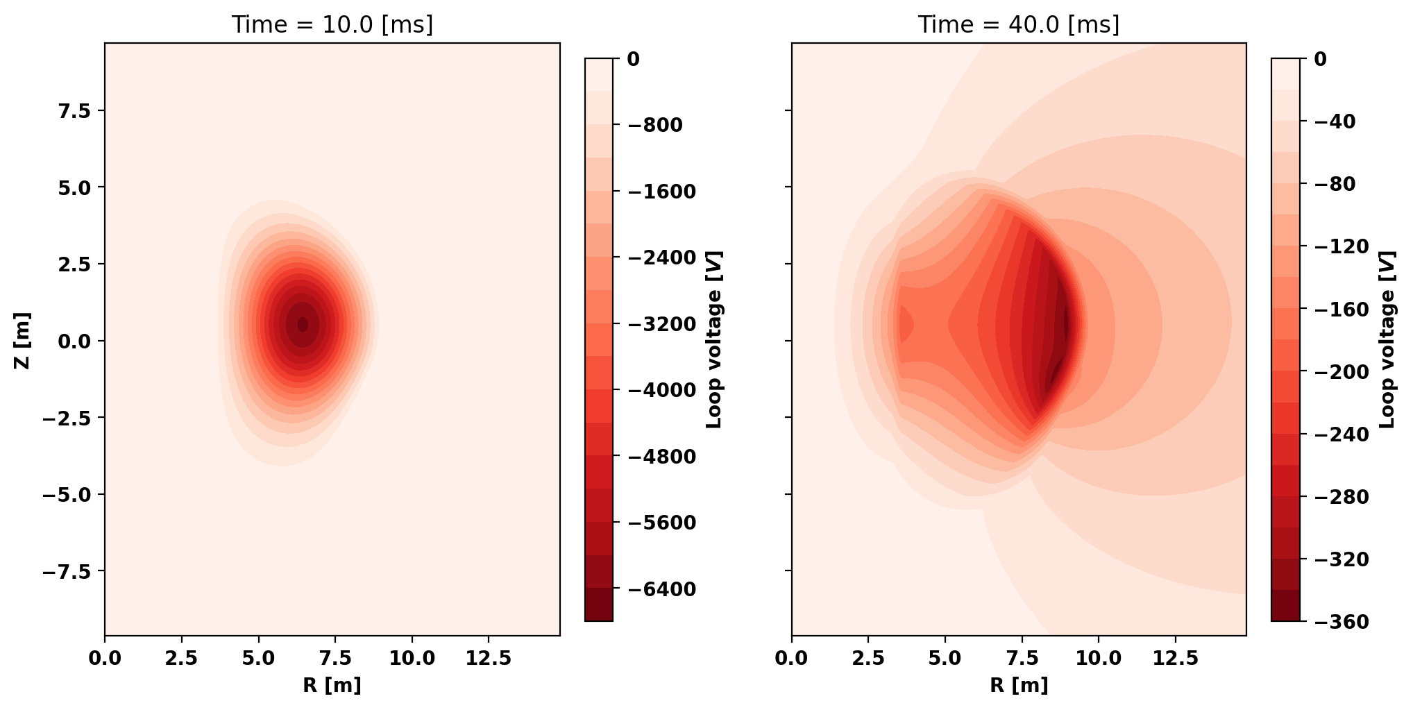
Plot loop voltage
fig, ax = plt.subplots(1,2,figsize=(10,5),sharey=True,constrained_layout=True)
dpsi_dt = (results[ind_sample+1]-results[ind_sample-1])/(sim_time[ind_sample+1]-sim_time[ind_sample-1])
clf = ax[0].tricontourf(mygs.r[:,0],mygs.r[:,1],mygs.lc,2.0*np.pi*dpsi_dt,levels=20,cmap='Reds_r')
fig.colorbar(clf,ax=ax[0],label=r'Loop voltage [$V$]', shrink=0.95)
ax[0].set_title('Time = {0:.1f} [ms]'.format(sim_time[ind_sample]*1.E3))
dpsi_dt = (results[ind_sample2+1]-results[ind_sample2-1])/(sim_time[ind_sample2+1]-sim_time[ind_sample2-1])
clf = ax[1].tricontourf(mygs.r[:,0],mygs.r[:,1],mygs.lc,2.0*np.pi*dpsi_dt,levels=20,cmap='Reds_r')
fig.colorbar(clf,ax=ax[1],label=r'Loop voltage [$V$]', shrink=0.95)
ax[1].set_title('Time = {0:.1f} [ms]'.format(sim_time[ind_sample2]*1.E3))
ax[0].set_ylabel('Z [m]')
ax[0].set_xlabel('R [m]')
_ = ax[1].set_xlabel('R [m]')
for ax_tmp in ax:
ax_tmp.set_aspect('equal','box')
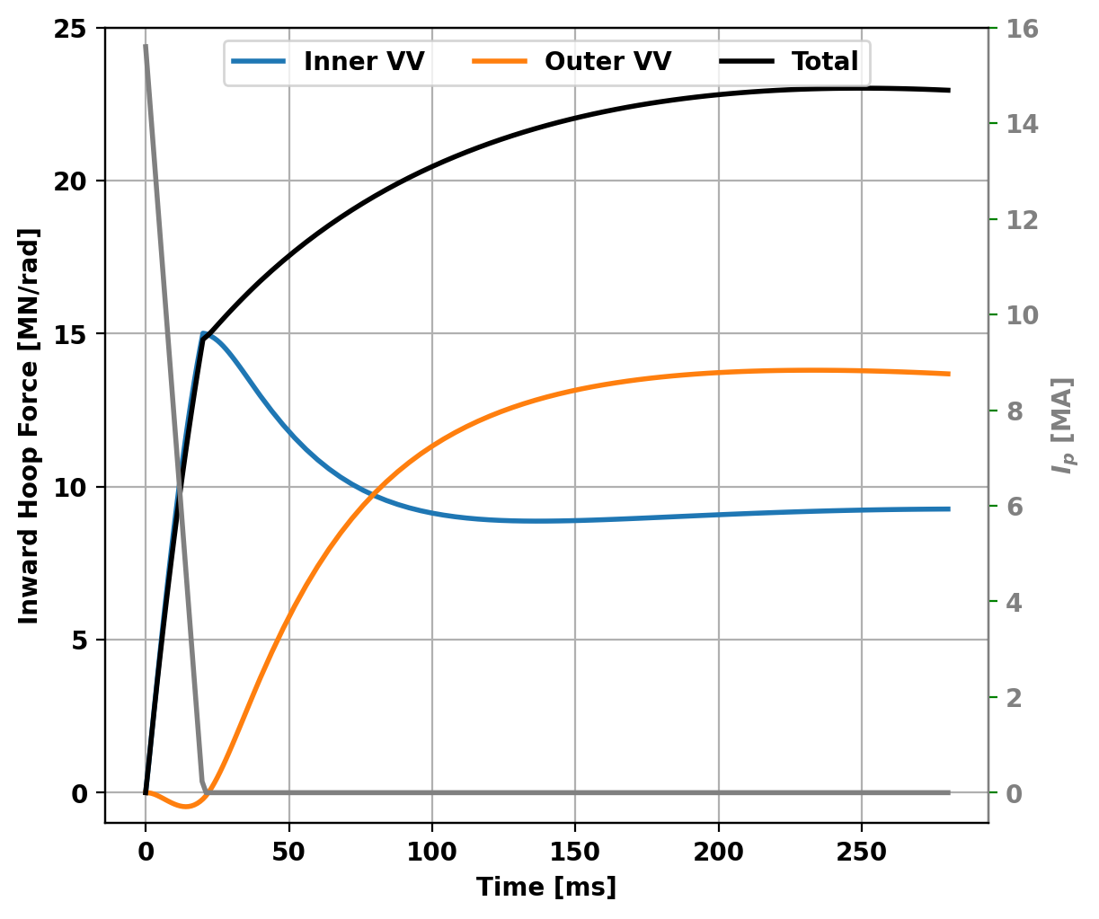
Compute and plot forces
Fr_inner = np.zeros((len(results),))
Fr_outer = np.zeros((len(results),))
for i, result in enumerate(results):
mesh_currents, Bv_cond, mask, rcc = compute_forces_components(mygs,results[i])
Fr_inner[i] = mygs.area_integral(mesh_currents*mygs.r[:,0]*Bv_cond[:,2],reg_mask=cond_dict['VV1']['reg_id'])
Fr_outer[i] = mygs.area_integral(mesh_currents*mygs.r[:,0]*Bv_cond[:,2],reg_mask=cond_dict['VV2']['reg_id'])
fig, ax = plt.subplots(1,1,figsize=(6,5),constrained_layout=True)
x = np.linspace(0.0,sim_time[-1]*1.E3,200)
y = np.zeros_like(x); y[x<CQ_time*1.E3] = (CQ_time*1.E3-x[x<CQ_time*1.E3])*Ip_target/1.E6/(CQ_time*1.E3)
ax2 = ax.twinx()
ax2.plot(x,y,label=r'$I_P$',color='0.5')
ax.plot(np.asarray(sim_time)*1.E3,-np.asarray(Fr_inner)/1.E6,label='Inner VV')
ax.plot(np.asarray(sim_time)*1.E3,-np.asarray(Fr_outer)/1.E6,label='Outer VV')
ax.plot(np.asarray(sim_time)*1.E3,-(np.asarray(Fr_inner)+np.asarray(Fr_outer))/1.E6,'k',label='Total')
ax.grid(True)
ax.set_ylim(-1,25)
ax2.set_ylim(-16/25.,16)
ax.legend(loc='upper center',ncols=3)
ax.set_ylabel(r'Inward Hoop Force [MN/rad]')
ax2.set_ylabel(r'$I_p$ [MA]',color='0.5')
ax2.tick_params(color='green', labelcolor='0.5')
ax2.spines['right'].set_edgecolor('0.5')
_ = ax.set_xlabel(r'Time [ms]')
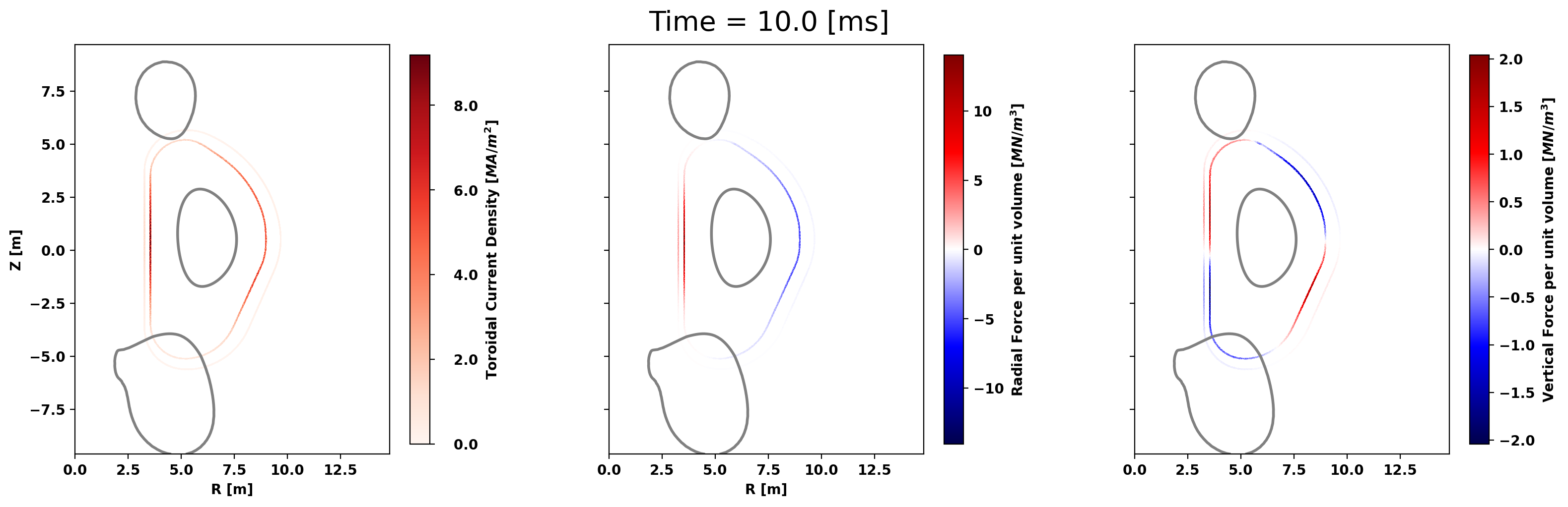
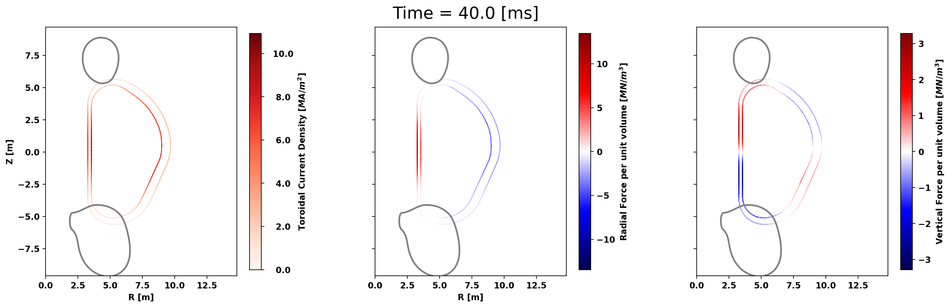
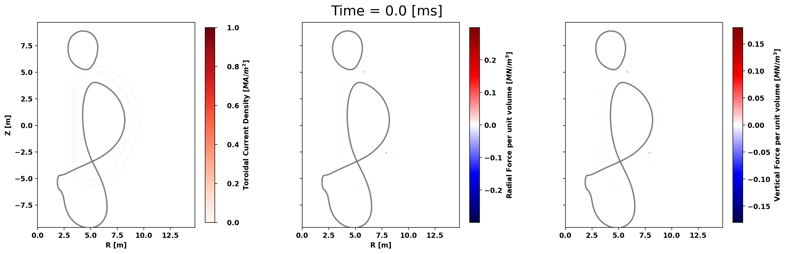
def plot_CQ(fig, ax, psi, time):
J_cond, Bv_cond, mask, rcc = compute_forces_components(mygs,psi,cell_centered=True)
Jphi = J_cond[mask]
Jphi /= 1.E6
vmax = max(1.E0,abs(Jphi).max())
mygs.plot_psi(fig,ax[0],psi=psi,normalized=False,plasma_levels=[psi_lim],plasma_color=['0.5'],vacuum_levels=None,xpoint_color=None,opoint_color=None)
clf2 = ax[0].tripcolor(mygs.r[:,0],mygs.r[:,1],mygs.lc[mask],Jphi,cmap='Reds', vmin=0.0, vmax=vmax)
cb1 = fig.colorbar(clf2,ax=ax[0],label=r'Toroidal Current Density [$MA/m^2$]',format='{x:6.1f}',shrink=0.95)
Fr = J_cond[mask]*Bv_cond[mask,2]
Fr /= 1.E6
vmax = abs(Fr).max()
mygs.plot_psi(fig,ax[1],psi=psi,normalized=False,plasma_levels=[psi_lim],plasma_color=['0.5'],vacuum_levels=None,xpoint_color=None,opoint_color=None)
clf = ax[1].tripcolor(mygs.r[:,0],mygs.r[:,1],mygs.lc[mask],Fr,cmap='seismic', vmin=-vmax, vmax=vmax)
cb2 = fig.colorbar(clf,ax=ax[1],label=r'Radial Force per unit volume [$MN/m^3$]', shrink=0.95)
Fz = -J_cond[mask]*Bv_cond[mask,0]
Fz /= 1.E6
vmax = abs(Fz).max()
mygs.plot_psi(fig,ax[2],psi=psi,normalized=False,plasma_levels=[psi_lim],plasma_color=['0.5'],vacuum_levels=None,xpoint_color=None,opoint_color=None)
clf = ax[2].tripcolor(mygs.r[:,0],mygs.r[:,1],mygs.lc[mask],Fz,cmap='seismic', vmin=-vmax, vmax=vmax)
cb3 = fig.colorbar(clf,ax=ax[2],label=r'Vertical Force per unit volume [$MN/m^3$]', shrink=0.95)
fig.suptitle('Time = {0:.1f} [ms]'.format(time*1.E3),fontsize=20)
ax[0].set_ylabel('Z [m]')
ax[0].set_xlabel('R [m]')
_ = ax[1].set_xlabel('R [m]')
for ax_tmp in ax:
ax_tmp.set_aspect('equal','box')
return cb1, cb2, cb3
fig, ax = plt.subplots(1,3,figsize=(16,5),sharey=True,constrained_layout=True)
_ = plot_CQ(fig, ax, results[ind_sample], sim_time[ind_sample])
fig, ax = plt.subplots(1,3,figsize=(16,5),sharey=True,constrained_layout=True)
_ = plot_CQ(fig, ax, results[ind_sample2], sim_time[ind_sample2])
Create animation of simulation
import matplotlib.animation
fig, ax = plt.subplots(1,3,figsize=(16,5),sharey=True,constrained_layout=True)
cbs = [None, None, None]
def animate(ii):
global cbs
for cb in cbs:
if cb is not None:
cb.remove()
for ax_tmp in ax:
ax_tmp.clear()
cbs[0], cbs[1], cbs[2] = plot_CQ(fig, ax, results[ii], sim_time[ii])
ani = matplotlib.animation.FuncAnimation(fig, animate, frames=40)
ani.save('ITER_CQ.gif',dpi=200,fps=10)