TokaMaker Meshing Example: Building a mesh for ITER

In this example we show how to generate a mesh for the ITER device using TokaMakers built in mesh generation.

Note

Running this example requires the h5py python packages, which is installable using pip or other standard methods.

import os
import sys
import json
import numpy as np
import matplotlib.pyplot as plt
plt.rcParams['figure.figsize']=(6,6)
plt.rcParams['font.weight']='bold'
plt.rcParams['axes.labelweight']='bold'
plt.rcParams['lines.linewidth']=2
plt.rcParams['lines.markeredgewidth']=2
%matplotlib inline
%config InlineBackend.figure_format = "retina"

Load TokaMaker library

To load the TokaMaker python module we need to tell python where to the module is located. This can be done either through the PYTHONPATH environment variable or using within a script using sys.path.append() as below, where we look for the environement variable OFT_ROOTPATH to provide the path to where the OpenFUSIONToolkit is installed (/Applications/OFT on macOS).

For meshing we will use the gs_Domain class to build a 2D triangular grid suitable for Grad-Shafranov equilibria. This class uses the triangle code through a simple internal python wrapper within OFT.

tokamaker_python_path = os.getenv('OFT_ROOTPATH')
if tokamaker_python_path is not None:
    sys.path.append(os.path.join(tokamaker_python_path,'python'))
from OpenFUSIONToolkit.TokaMaker.meshing import gs_Domain, save_gs_mesh

Build mesh

Set mesh resolution for each region

First we define some target sizes to set the resolution in out grid. These variables will be used later and represent the target edge size within a given region, where units are in meters. In this case we are using a fairly coarse resolution of 15 cm in the plasma region and 60 cm in the vacuum region. Note that when setting up a new machine these values will need to scale with the overall size of the device/domain. Additionally, one should perform a convergence study, by increasing resolution (decreasing target size) by at least a factor of two in all regions to ensure the results are not sensitive to your choice of grid size.

plasma_dx = 0.15
coil_dx = 0.2
vv_dx = 0.3
vac_dx = 0.6

Load geometry information

The geometry information (eg. bounding curves for vacuum vessels) are now loaded from a JSON file. For simple geometries, testing, or generative usage this can be created directly in the code. However, it is often helpful to separate this information into a fixed datafile as here. This JSON file contains the following:

• limiter: A contour of R,Z points defining the limiter (PFC) surface
• inner_vv: Two contours of R,Z points defining the inner and outer boundary of the inner vacuum vessel
• outer_vv: Two contours of R,Z points defining the inner and outer boundary of the outer vacuum vessel
• coils: A dictionary of R,Z,W,H values defining the PF coils as rectangles in the poloidal cross-section

with open('ITER_geom.json','r') as fid:
    ITER_geom = json.load(fid)

Define regions and attributes

We now create and define the various logical mesh regions. In the ITER case we have 6 regions:

• air: The region outside the vacuum vessel, which is not actually air in a complex device like ITER but we use this terminology for commonality with present research devices
• plasma: The region inside the limiter where the plasma will exist
• vacuum1: The region between the inner vacuum vessel and the limiter
• vacuum2: The region between the inner and outer vacuum vessels
• vv1: The inner vacuum vessel
• vv2: The outer vacuum vessel
• PF1,...: Each of the 14 coils in ITER (6 CS, 6 PF, 2 VS)

In ITER all coils are independent except for the vertical stability coil (VS), which is single coil set composed of two counter-wound coils. To treat this set as a single coil we use the coil_set and nTurns argument to define_region() to join the coils in a single VS coil set with opposing polarities.

Note

nTurns can also be used to define the number of turns in a given coil region. At the moment we are not including # of turns in this model so we keep the amplitude for each coil as 1.0 and only adjust the polarity.

For each region you can provide a target size and one of four region types:

• plasma: The region where the plasma can exist and the classic Grad-Shafranov equation with \(F*F'\) and \(P'\) are allowed. There can only be one region of this type
• vacuum: A region where not current can flow and \(\nabla^* \psi = 0\) is solved
• boundary: A special case of the vacuum region, which forms the outer boundary of the computational domain. A region of this type is required if more than one region is specified
• conductor: A region where toroidal current can flow passively (no externally applied voltage). For this type of region the resistivity should be specified with the argument eta in units of \(\omega \mathrm{-m}\).
• coil: A region where toroidal current can flow with specified amplitude through set_coil_currents() or via shape optimization set_coil_reg() and set_isoflux()

# Create a G-S domain
gs_mesh = gs_Domain()
# Define region information for mesh
gs_mesh.define_region('air',vac_dx,'boundary')
gs_mesh.define_region('plasma',plasma_dx,'plasma')
gs_mesh.define_region('vacuum1',vv_dx,'vacuum',allow_xpoints=True)
gs_mesh.define_region('vacuum2',vv_dx,'vacuum')
gs_mesh.define_region('vv1',vv_dx,'conductor',eta=6.9E-7)
gs_mesh.define_region('vv2',vv_dx,'conductor',eta=6.9E-7)
# Define each of the PF coils
for key, coil in ITER_geom['coils'].items():
    if not key.startswith('VS'):
        gs_mesh.define_region(key,coil_dx,'coil')
gs_mesh.define_region('VSU',coil_dx,'coil',coil_set='VS',nTurns=1.0)
gs_mesh.define_region('VSL',coil_dx,'coil',coil_set='VS',nTurns=-1.0)

Define geometry for region boundaries

Once the region types and properties are defined we now define the geometry of the mesh using shapes and references to the defined regions.

1. We add the limiter contour as a "polygon", referencing plasma as the region enclosed by the contour and vacuum1 as the region outside the contour.
2. We add the inner vacuum vessel as an "annulus" with curves defining the inner and outer edges respectively. We also reference vacuum1 as the region enclosed by the annulus, vv1 as the annular region itself, and vacuum2 as the region outside the annulus.
3. We add the outer vacuum vessel as an "annulus" with curves defining the inner and outer edges respectively. We also reference vacuum2 as the region enclosed by the annulus, vv2 as the annular region itself, and air as the region outside the annulus.
4. We add each of the 14 coils as "rectangles", which are defined by a center point (R,Z) along with a width (W) and height (H). We also reference air as the region outside the rectangle for the CS and PF coils and vacuum1 for the VS coils.

# Define geometry
gs_mesh.add_polygon(ITER_geom['limiter'],'plasma',parent_name='vacuum1')             # Define the shape of the limiter
gs_mesh.add_annulus(ITER_geom['inner_vv'][0],'vacuum1',ITER_geom['inner_vv'][1],'vv1',parent_name='vacuum2') # Define the shape of the VV
gs_mesh.add_annulus(ITER_geom['outer_vv'][0],'vacuum2',ITER_geom['outer_vv'][1],'vv2',parent_name='air') # Define the shape of the VV
# Define the shape of the PF coils
for key, coil in ITER_geom['coils'].items():
    if key.startswith('VS'):
        gs_mesh.add_rectangle(coil['rc'],coil['zc'],coil['w'],coil['h'],key,parent_name='vacuum1')
    else:
        gs_mesh.add_rectangle(coil['rc'],coil['zc'],coil['w'],coil['h'],key,parent_name='air')

  Warning: sliver (angle=45.0) detected at point 31 (5.565, -4.5559)

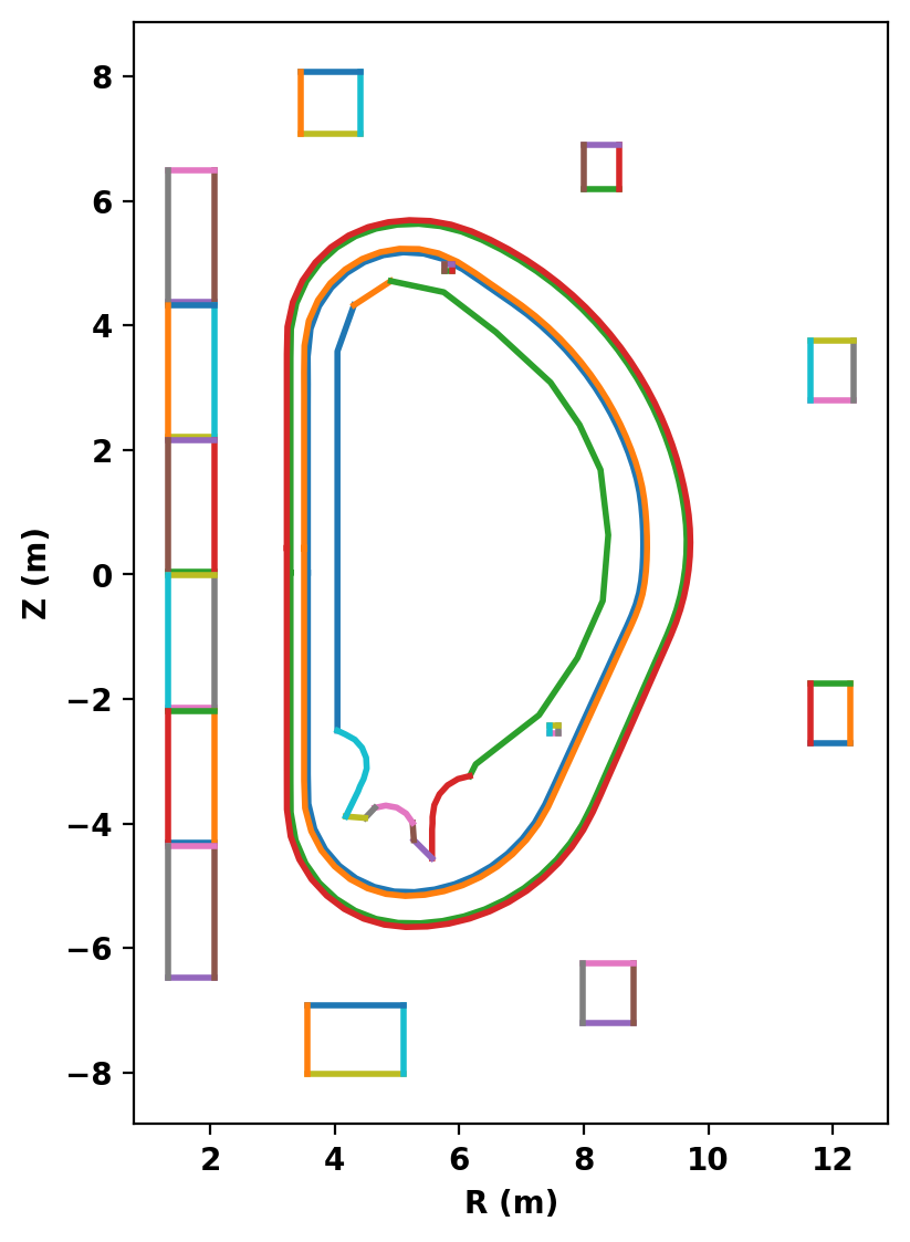
Plot topology

After defining the logical and physical topology we can now plot the curves within the definitions to double check everything is in the right place. In cases where curves appear to cross eachother (as with the VS coil and inner VV) one should zoom in to ensure no crossings exist. In this case we had to move the upper VS coil down by 1 cm to avoid an intersection with the geometry available for this example.

fig, ax = plt.subplots(1,1,figsize=(4,6),constrained_layout=True)
gs_mesh.plot_topology(fig,ax)

Create mesh

Now we generate the actual mesh using the build_mesh() method. Additionally, if coil and/or conductor regions are defined the get_coils() and get_conductors() methods should also be called to get descriptive dictionaries for later use in TokaMaker. This step may take a few moments as triangle generates the mesh.

Note that, as is common with unstructured meshes, the mesh is stored a list of points mesh_pts of size (np,2), a list of cells formed from three points each mesh_lc of size (nc,3), and an array providing a region id number for each cell mesh_reg of size (nc,), which is mapped to the names above using the coil_dict and cond_dict dictionaries.

mesh_pts, mesh_lc, mesh_reg = gs_mesh.build_mesh()
coil_dict = gs_mesh.get_coils()
cond_dict = gs_mesh.get_conductors()

Assembling regions:
  # of unique points    = 885
  # of unique segments  = 74
Generating mesh:
  # of points  = 4757
  # of cells   = 9400
  # of regions = 20

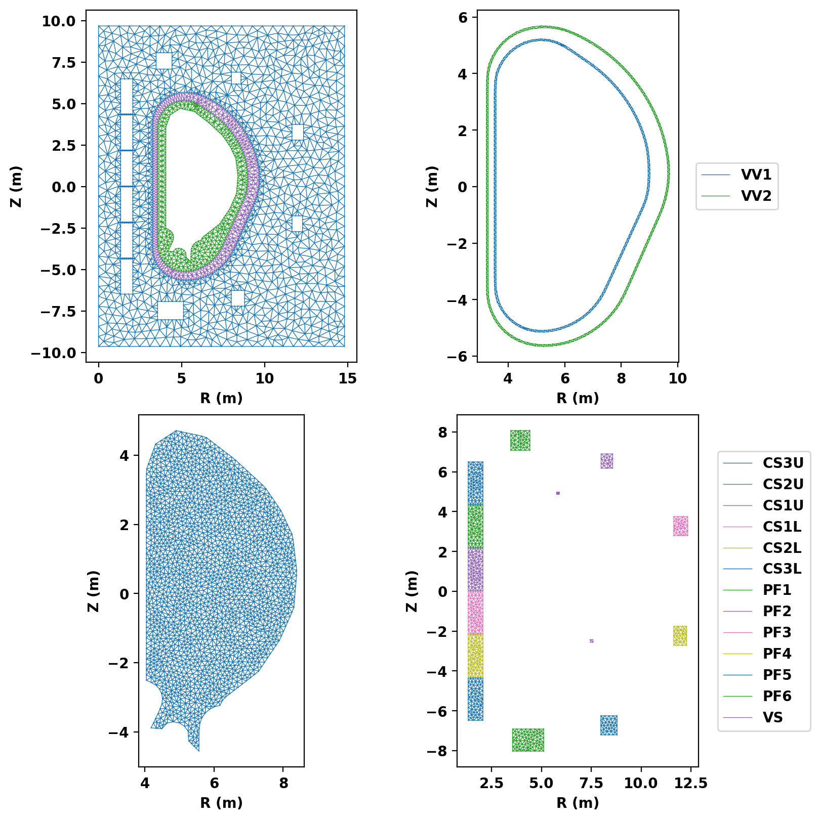
Plot resulting regions and grid

We now plot the mesh by region to inspect proper generation.

fig, ax = plt.subplots(2,2,figsize=(8,8),constrained_layout=True)
gs_mesh.plot_mesh(fig,ax)

Save mesh for later use

As generation of the mesh often takes comparable, or longer, time compare to runs in TokaMaker it is useful to separate generation of the mesh into a different script as demonstrated here. The method save_gs_mesh() can be used to save the resulting information for later use. This is done using and an HDF5 file through the h5py library.

save_gs_mesh(mesh_pts,mesh_lc,mesh_reg,coil_dict,cond_dict,'ITER_mesh.h5')