In this example we show how to perform an equilibrium reconstruction in ITER from a simple with L-mode case

This example utilizes the mesh built in TokaMaker Meshing Example: Building a mesh for ITER.

Note: Running this example requires the h5py python package, which is installable using pip or other standard methods.

Warning: The reconstruction functionality in TokaMaker is still a work in progress, as the PSI-Tri capabilities are activated and tested. Please use with care.

import os
import sys
import json
import random
import numpy as np
import matplotlib.pyplot as plt
plt.rcParams['figure.figsize']=(6,6)
plt.rcParams['font.weight']='bold'
plt.rcParams['axes.labelweight']='bold'
plt.rcParams['lines.linewidth']=2
plt.rcParams['lines.markeredgewidth']=2
%matplotlib inline
%config InlineBackend.figure_format = "retina"

Load TokaMaker library

To load the TokaMaker python module we need to tell python where to the module is located. This can be done either through the PYTHONPATH environment variable or using within a script using sys.path.append() as below, where we look for the environement variable OFT_ROOTPATH to provide the path to where the OpenFUSIONToolkit is installed (/Applications/OFT on macOS).

For meshing we will use the gs_Domain class to build a 2D triangular grid suitable for Grad-Shafranov equilibria. This class uses the triangle code through a python wrapper.

tokamaker_python_path = os.getenv('OFT_ROOTPATH')
if tokamaker_python_path is not None:
    sys.path.append(os.path.join(tokamaker_python_path,'python'))
from OpenFUSIONToolkit import OFT_env
from OpenFUSIONToolkit.TokaMaker import TokaMaker
from OpenFUSIONToolkit.TokaMaker.meshing import load_gs_mesh
from OpenFUSIONToolkit.TokaMaker.reconstruction import reconstruction
from OpenFUSIONToolkit.TokaMaker.util import create_power_flux_fun

Initialize TokaMaker object

We now create a OFT_env instance for execution using two threads and a TokaMaker instance to use for equilibrium calculations. Note at present only a single TokaMaker instance can be used per python kernel, so this command should only be called once in a given Jupyter notebook or python script. In the future this restriction may be relaxed.

myOFT = OFT_env(nthreads=2)

mygs = TokaMaker(myOFT)

#----------------------------------------------
Open FUSION Toolkit Initialized
Development branch:   v1_beta6
Revision id:          681e857
Parallelization Info:
  # of MPI tasks      =    1
  # of NUMA nodes     =    1
  # of OpenMP threads =    2
Fortran input file    = /var/folders/52/n5qxh27n4w19qxzqygz2btbw0000gn/T/oft_64714/oftpyin
XML input file        = none
Integer Precisions    =    4   8
Float Precisions      =    4   8  16
Complex Precisions    =    4   8
LA backend            = native
#----------------------------------------------

Load mesh into TokaMaker

Now we load the mesh generated in TokaMaker Meshing Example: Building a mesh for ITER using load_gs_mesh() and setup_mesh. Then we use setup_regions(), passing the conductor and coil dictionaries for the mesh, to define the different region types. Finally, we call setup() to setup the required solver objects. During this call we can specify the desired element order (min=2, max=4) and the toroidal field through F0 = B0*R0, where B0 is the toroidal field at a reference location R0.

mesh_pts,mesh_lc,mesh_reg,coil_dict,cond_dict = load_gs_mesh('ITER_mesh.h5')
mygs.setup_mesh(mesh_pts, mesh_lc, mesh_reg)
mygs.setup_regions(cond_dict=cond_dict,coil_dict=coil_dict)
mygs.setup(order = 2, F0 = 5.3*6.2)

**** Loading OFT surface mesh

**** Generating surface grid level  1
  Generating boundary domain linkage
  Mesh statistics:
    Area         =  2.859E+02
    # of points  =    4757
    # of edges   =   14156
    # of cells   =    9400
    # of boundary points =     112
    # of boundary edges  =     112
    # of boundary cells  =     112
  Resolution statistics:
    hmin =  9.924E-03
    hrms =  2.826E-01
    hmax =  8.466E-01
  Surface grounded at vertex     870


**** Creating Lagrange FE space
  Order  =    2
  Minlev =   -1

 Computing flux BC matrix 
 Inverting real matrix
   Time =    1.0939999999999999E-003

Define a vertical stability coil

Like many elongated equilibria, the equilibrium we seek to compute below is vertically unstable. In this case we use the actual ITER Vertical Stability Coil (VSC) in order to help with convergence using the set_coil_vsc() method.

Note: While ITER has a "real" VSC, this is not required and this functionality can instead be used to define a "virtual" VSC by pairing coils in a way that are not necessarily paired experimentally.

mygs.set_coil_vsc({'VS': 1.0})

Define hard limits on coil currents

Hard limits on coil currents can be set using set_coil_bounds(). In this case we just the simple and approximate bi-directional limit of 50 MA in each coil.

Bounds are specified using a dictionary of 2 element lists, containing the minimum and maximum bound, where the dictionary key corresponds to the coil names, which are available in mygs.coil_sets

coil_bounds = {key: [-50.E6, 50.E6] for key in mygs.coil_sets}

mygs.set_coil_bounds(coil_bounds)

Compute Equilibrium for Reconstruction

Define global quantities and targets

For the inverse case we define a target for the plasma current and the peak plasma pressure, which occurs on the magnetic axis.

Note: These constraints can be considered "hard" constraints, where they will be matched to good tolerance as long as the calculation converges.

Ip_target=15.6E6
P0_target=6.2E5
mygs.set_targets(Ip=Ip_target, pax=P0_target)

Define shape targets

In order to constrain the shape of the plasma we can utilize two types of constraints:

isoflux points, which are points we want to lie on the same flux surface (eg. the LCFS)
saddle points, where we want the poloidal magnetic field to vanish (eg. X-points). While one can also use this constraint to enforce a magnetic axis location, instead set_targets() should be used with arguments R0 and V0.

Note: These constraints can be considered "soft" constraints, where the calculation attempts to minimize error in satisfying these constraints subject to other constraints and regularization.

Here we define a handful of isoflux points that we want to lie on the LCFS of the target equilibrium. Additionally, we define a single X-point and set it as a saddle constraint as well as adding it to the list of isoflux points.

isoflux_pts = np.array([
    [ 8.20,  0.41],
    [ 8.06,  1.46],
    [ 7.51,  2.62],
    [ 6.14,  3.78],
    [ 4.51,  3.02],
    [ 4.26,  1.33],
    [ 4.28,  0.08],
    [ 4.49, -1.34],
    [ 7.28, -1.89],
    [ 8.00, -0.68]
])
x_point = np.array([[5.125, -3.4],])
mygs.set_isoflux(np.vstack((isoflux_pts,x_point)))
mygs.set_saddles(x_point)

Define coil regularization matrix

In general, for a given coil set a given plasma shape cannot be exactly reproduced, which generally yields large amplitude coil currents if no constraint on the coil currents is applied. As a result, it is useful to include regularization terms for the coils to balance minimization of the shape error with the amplitude of current in the coils. In TokaMaker these regularization terms have the general form, where each term corresponds to a set of coil coefficients, target value, and weight. The coil_reg_term() method is provided to aid in defining these terms.

In this case, one regularization term is added for each coil with a single unit coefficient for that coil and target of zero with modest weights. This regularization acts to penalize the amplitude of current in each coil, acting to balance coil current with error in the shape targets. Note that the weight on the VSC virtual coil (#VSC) defined above is set high to prevent interaction with the real VS coil set (see below for further information).

# Set regularization weights
regularization_terms = []
for name, coil in mygs.coil_sets.items():
    # Set zero target current and different small weights to help conditioning of fit
    if name.startswith('CS'):
        if name.startswith('CS1'):
            regularization_terms.append(mygs.coil_reg_term({name: 1.0},target=0.0,weight=2.E-2))
        else:
            regularization_terms.append(mygs.coil_reg_term({name: 1.0},target=0.0,weight=1.E-2))
    elif name.startswith('PF'):
        regularization_terms.append(mygs.coil_reg_term({name: 1.0},target=0.0,weight=1.E-2))
    elif name.startswith('VS'):
        regularization_terms.append(mygs.coil_reg_term({name: 1.0},target=0.0,weight=1.E-2))
# Disable VSC virtual coil
regularization_terms.append(mygs.coil_reg_term({'#VSC': 1.0},target=0.0,weight=1.E2))
 
# Pass regularization terms to TokaMaker
mygs.set_coil_reg(reg_terms=regularization_terms)

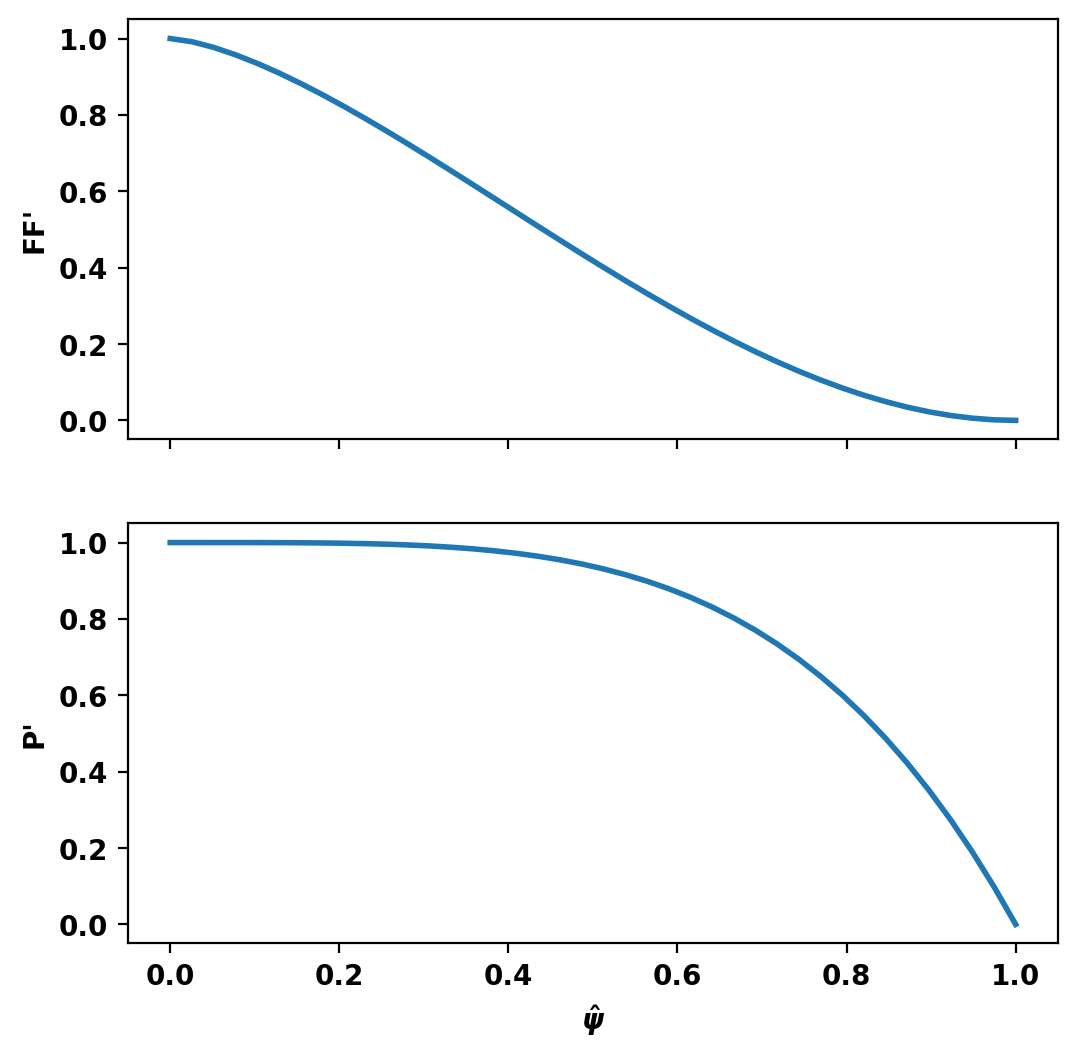
Define flux functions

Although TokaMaker has a "default" profile for the F*F' and P' terms this should almost never be used and one should instead choose an appropriate flux function for their application. In this case we use an L-mode-like profile of the form \(((1-\hat{\psi})^{\alpha})^{\gamma}\), using create_power_flux_fun(), where \(\alpha\) and \(\gamma\) are set differently for F*F' and P' to provide peaked and broad profiles respectively. Within TokaMaker this profile is represented as a piecewise linear function, which can be set up using the dictionary approach shown below.

# Set profiles
ffp_prof = create_power_flux_fun(40,1.5,2.0)
pp_prof = create_power_flux_fun(40,4.0,1.0)
 
fig, ax = plt.subplots(2,1,sharex=True)
# Plot F*F'
ax[0].plot(ffp_prof['x'],ffp_prof['y'])
ax[0].set_ylabel("FF'")
# Plot P'
ax[1].plot(pp_prof['x'],pp_prof['y'])
ax[1].set_ylabel("P'")
_ = ax[-1].set_xlabel(r"$\hat{\psi}$")
 
mygs.set_profiles(ffp_prof=ffp_prof,pp_prof=pp_prof)

Compute equilibrium

We can now compute a free-boundary equilibrium using these constraints. Note that before running a calculation for the first time we must initialize the flux function \(\psi\), which can be done using init_psi(). This subroutine initializes the flux using the specified Ip_target from above, which is evenly distributed over the entire plasma region or only with a boundary defined using a center point (R,Z), minor radius (a), and elongation and triangularity. Coil currents are also initialized at this point using the constraints above and this uniform plasma current initialization.

solve() is then called to compute a self-consitent Grad-Shafranov equilibrium. If the result variable (err_flag) is zero then the solution has converged to the desired tolerance ( \(10^{-6}\) by default).

R0 = 6.3
Z0 = 0.5
a = 2.0
kappa = 1.4
delta = 0.0
mygs.init_psi(R0, Z0, a, kappa, delta)
mygs.solve()

Starting non-linear GS solver
     1  5.7965E+00  1.5693E-01  6.4686E-01  6.4422E+00  5.3430E-01  9.8316E-04
     2  1.5480E+01  9.5055E-02  2.7469E-01  6.4072E+00  5.3290E-01  1.5938E-03
     3  1.9148E+01  7.9379E-02  1.2986E-01  6.3868E+00  5.3264E-01  1.6630E-03
     4  2.0951E+01  7.3407E-02  6.7604E-02  6.3757E+00  5.3235E-01  1.6305E-03
     5  2.1908E+01  7.0680E-02  3.6983E-02  6.3697E+00  5.3227E-01  1.5882E-03
     6  2.2433E+01  6.9312E-02  2.0669E-02  6.3664E+00  5.3231E-01  1.5557E-03
     7  2.2724E+01  6.8590E-02  1.1653E-02  6.3646E+00  5.3240E-01  1.5342E-03
     8  2.2888E+01  6.8198E-02  6.5944E-03  6.3636E+00  5.3250E-01  1.5207E-03
     9  2.2980E+01  6.7980E-02  3.7379E-03  6.3631E+00  5.3258E-01  1.5126E-03
    10  2.3032E+01  6.7859E-02  2.1210E-03  6.3628E+00  5.3265E-01  1.5079E-03
    11  2.3061E+01  6.7791E-02  1.2045E-03  6.3626E+00  5.3270E-01  1.5051E-03
    12  2.3078E+01  6.7753E-02  6.8471E-04  6.3625E+00  5.3274E-01  1.5035E-03
    13  2.3087E+01  6.7731E-02  3.8962E-04  6.3625E+00  5.3277E-01  1.5025E-03
    14  2.3093E+01  6.7719E-02  2.2195E-04  6.3624E+00  5.3279E-01  1.5020E-03
    15  2.3096E+01  6.7712E-02  1.2660E-04  6.3624E+00  5.3280E-01  1.5017E-03
    16  2.3097E+01  6.7708E-02  7.2329E-05  6.3624E+00  5.3281E-01  1.5015E-03
    17  2.3098E+01  6.7705E-02  4.1395E-05  6.3624E+00  5.3281E-01  1.5014E-03
    18  2.3099E+01  6.7704E-02  2.3741E-05  6.3624E+00  5.3282E-01  1.5013E-03
    19  2.3099E+01  6.7703E-02  1.3650E-05  6.3624E+00  5.3282E-01  1.5013E-03
    20  2.3099E+01  6.7703E-02  7.8710E-06  6.3624E+00  5.3282E-01  1.5013E-03
    21  2.3100E+01  6.7703E-02  4.5542E-06  6.3624E+00  5.3282E-01  1.5013E-03
    22  2.3100E+01  6.7702E-02  2.6456E-06  6.3624E+00  5.3283E-01  1.5013E-03
    23  2.3100E+01  6.7702E-02  1.5440E-06  6.3624E+00  5.3283E-01  1.5013E-03
    24  2.3100E+01  6.7702E-02  9.0578E-07  6.3624E+00  5.3283E-01  1.5013E-03
 Timing:  0.20457699999678880     
   Source:     9.0972999634686857E-002
   Solve:      6.2907999963499606E-002
   Boundary:   5.3660001722164452E-003
   Other:      4.5330000226385891E-002

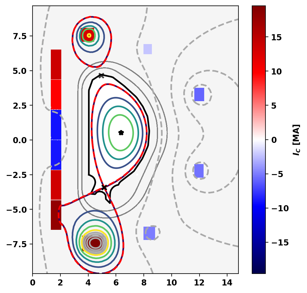
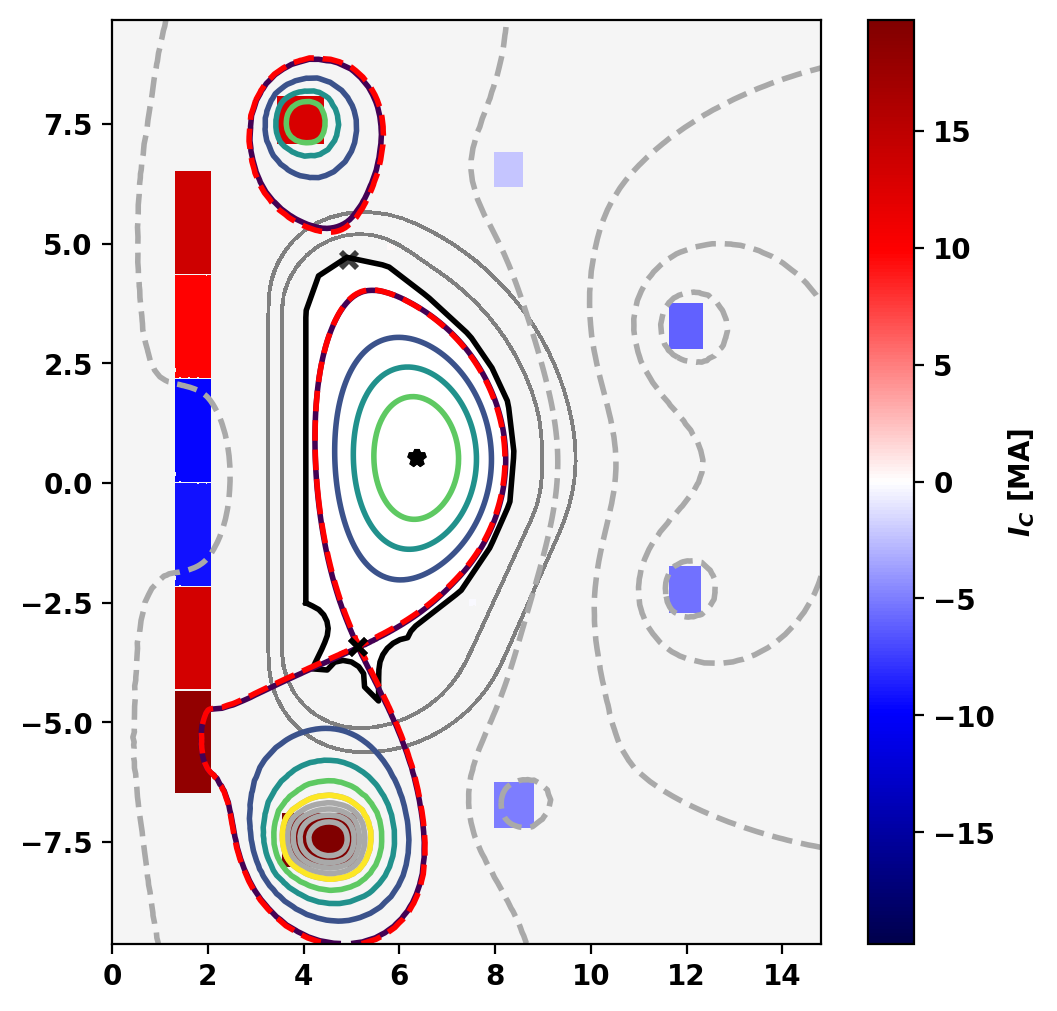
Plot equilibrium

Flux surfaces of the computed equilibrium can be plotted using the plot_psi() method. The additional plotting methods plot_machine() and plot_constraints() are also used to show context and other information. Each method has a large number of optional arguments for formatting and other options.

fig, ax = plt.subplots(1,1)
mygs.plot_machine(fig,ax,coil_colormap='seismic',coil_symmap=True,coil_scale=1.E-6,coil_clabel=r'$I_C$ [MA]')
mygs.plot_psi(fig,ax,xpoint_color=None,vacuum_nlevels=4)
mygs.plot_constraints(fig,ax,isoflux_color='tab:red',isoflux_marker='o')
psi_target = mygs.get_psi()
eq_target = mygs.get_stats()

Print equilibrium information and coil currents

Basic parameters can be displayed using the print_info() method. For access to these quantities as variables instead the get_stats() can be used.

The final coil currents can also be retrieved using the get_coil_currents() method, which are all within the approximate coil limits imposed above.

mygs.print_info()
 
print()
print("Coil Currents [MA]:")
coil_currents, _ = mygs.get_coil_currents()
for key, current in coil_currents.items():
    print('  {0:10} {1:10.2F}'.format(key+":",current/1.E6))

Equilibrium Statistics:
  Topology                =   Diverted
  Toroidal Current [A]    =    1.5600E+07
  Current Centroid [m]    =    6.203  0.530
  Magnetic Axis [m]       =    6.362  0.533
  Elongation              =    1.875 (U:  1.763, L:  1.987)
  Triangularity           =    0.477 (U:  0.405, L:  0.550)
  Plasma Volume [m^3]     =   820.079
  q_0, q_95               =    0.823  2.760
  Plasma Pressure [Pa]    =   Axis:  6.1923E+05, Peak:  6.1923E+05
  Stored Energy [J]       =    2.4299E+08
  <Beta_pol> [%]          =   42.6829
  <Beta_tor> [%]          =    1.7801
  <Beta_n>   [%]          =    1.1953
  Diamagnetic flux [Wb]   =    1.5403E+00
  Toroidal flux [Wb]      =    1.2187E+02
  l_i                     =    1.1597

Coil Currents [MA]:
  CS3U:           13.74
  CS2U:            9.74
  CS1U:           -9.06
  CS1L:           -8.81
  CS2L:           13.40
  CS3L:           17.88
  PF1:            12.94
  PF2:            -2.20
  PF3:            -5.95
  PF4:            -5.14
  PF5:            -5.18
  PF6:            19.93
  VS:              0.15

Perform Reconstruction

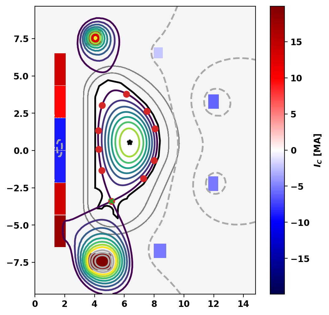
Define diagnostic set

For this example we define a simple set of flux loops and Mirnov sensors that lie on the inner vaccum vessel. The signal in these sensors will be used to constrain the reconstruction along with coil currents and global plasma quantities (eg. \(I_p\)).

# Load VV geometry
with open('ITER_geom.json','r') as fid:
    ITER_geom = json.load(fid)
    probe_contour = np.asarray(ITER_geom['inner_vv'][0])
# Rediscretize evenly in arc length
dl_contour = np.r_[0.0, np.cumsum(np.linalg.norm(np.diff(probe_contour,axis=0),axis=1))]
probe_contour_new = np.zeros((100,2))
probe_contour_new[:,0] = np.interp(np.linspace(0.0,dl_contour[-1],100),dl_contour,probe_contour[:,0])
probe_contour_new[:,1] = np.interp(np.linspace(0.0,dl_contour[-1],100),dl_contour,probe_contour[:,1])
# Place 20 probe locations evenly on contour
B_locs = []
for i, pt in enumerate(probe_contour_new):
    if i % 5 == 0:
        B_locs.append(pt)
B_locs = np.asarray(B_locs)

Plot equilibrium and probe locations

fig, ax = plt.subplots(1,1)
mygs.plot_machine(fig,ax,coil_colormap='seismic',coil_scale=1.E-6,coil_clabel=r'$I_C$ [MA]',coil_symmap=True)
mygs.plot_psi(fig,ax,plasma_nlevels=5,vacuum_nlevels=5)
mygs.plot_constraints(fig, ax)
ax.plot(B_locs[:,0], B_locs[:,1], 'o')

[<matplotlib.lines.Line2D at 0x11ffe8550>]

Create reconstruction object

myrecon = reconstruction(mygs)

Set plasma current constraint

First we define a constraint on the plasma current with 5% random noise added to the signal and an appropriate error. This constraint is equivalent to the measurement of a synthetic Rigowskii coil and can be set using set_Ip().

noise_amp = (random.random()-0.5)*2.0
Ip_noised = eq_target['Ip']*(1.0+noise_amp*0.05)
myrecon.set_Ip(Ip_noised, err=0.05*eq_target['Ip'])

Set flux loop constraints

Next we sample the poloidal flux at each of the locations defined above with 5% random noise added to each signal. Flux loop constraints are defined using add_flux_loop().

Note: Poloidal flux and \(\psi\) differ by a factor of \(2 \pi\) that must be accounted for when computing synthetic flux loop signals.

flux_vals = []
field_eval = mygs.get_field_eval('PSI')
for i in range(B_locs.shape[0]):
    B_tmp = field_eval.eval(B_locs[i,:])
    noise_amp = (random.random()-0.5)*2.0
    flux_vals.append(B_tmp[0])
    psi_val = B_tmp[0]*2.0*np.pi
    myrecon.add_flux_loop(B_locs[i,:], psi_val*(1.0 + noise_amp*0.05), err=abs(psi_val*0.05))

Set Mirnov constraints

Next we sample the radial and vertical magnetic field at each of the locations defined above with 5% random noise added to each signal. Local B-field constraints are defined using add_Mirnov().

field_eval = mygs.get_field_eval('B')
for i in range(B_locs.shape[0]):
    B_tmp = field_eval.eval(B_locs[i,:])
    noise_amp = (random.random()-0.5)*2.0
    myrecon.add_Mirnov(B_locs[i,:], np.r_[1.0,0.0,0.0], B_tmp[0] + noise_amp*abs(B_tmp[0]*0.05), err=abs(B_tmp[0]*0.05))
    noise_amp = (random.random()-0.5)*2.0
    myrecon.add_Mirnov(B_locs[i,:], np.r_[0.0,0.0,1.0], B_tmp[2] + noise_amp*abs(B_tmp[2]*0.05), err=abs(B_tmp[2]*0.05))

Add noise to coil currents

coil_currents, _ = mygs.get_coil_currents()
for key in coil_currents:
    noise_amp = (random.random()-0.5)*2.0
    coil_currents[key] *= 1.0+noise_amp*0.05

Compute starting equilibrium

# Replace shape constraints with absolute flux and current constraints
mygs.set_isoflux(None)
mygs.set_saddles(None)
mygs.set_targets(Ip=Ip_noised,Ip_ratio=2.0)
mygs.set_flux(B_locs,np.array(flux_vals))
 
# Set coil regularization to weakly track measured coil currents
regularization_terms = []
for name in coil_currents:
    regularization_terms.append(mygs.coil_reg_term({name: 1.0},target=coil_currents[name],weight=1.E-1))
regularization_terms.append(mygs.coil_reg_term({'#VSC': 1.0},target=0.0,weight=1.E2))
 
# Pass regularization terms to TokaMaker
mygs.set_coil_reg(reg_terms=regularization_terms)
 
# Initial equilibrium with very rough guess
R0 = 6.3
Z0 = 0.5
a = 1.0
kappa = 1.0
delta = 0.0
err_flag = mygs.init_psi(R0, Z0, a, kappa, delta)
 
# Update maximum number of solver iterations
mygs.settings.maxits=100
mygs.update_settings()
 
# Compute initial equilibrium
mygs.solve()

Starting non-linear GS solver
     1  2.3496E+01  8.2426E-02  9.5926E-02  6.3385E+00  5.0369E-01  1.2320E-01
     2  2.3331E+01  7.6491E-02  4.0608E-02  6.3461E+00  5.0101E-01  8.2651E-02
     3  2.3123E+01  7.4775E-02  1.8982E-02  6.3542E+00  5.0058E-01  6.0447E-02
     4  2.3039E+01  7.4161E-02  9.6013E-03  6.3607E+00  5.0131E-01  4.7738E-02
     5  2.3013E+01  7.3909E-02  5.1273E-03  6.3653E+00  5.0258E-01  4.0462E-02
     6  2.3007E+01  7.3788E-02  2.8748E-03  6.3684E+00  5.0406E-01  3.6243E-02
     7  2.3008E+01  7.3721E-02  1.6998E-03  6.3704E+00  5.0556E-01  3.3751E-02
     8  2.3008E+01  7.3678E-02  1.0753E-03  6.3717E+00  5.0700E-01  3.2238E-02
     9  2.3007E+01  7.3647E-02  7.4406E-04  6.3726E+00  5.0835E-01  3.1282E-02
    10  2.3005E+01  7.3623E-02  5.6856E-04  6.3731E+00  5.0960E-01  3.0647E-02
    11  2.3002E+01  7.3603E-02  4.7133E-04  6.3734E+00  5.1074E-01  3.0203E-02
    12  2.2999E+01  7.3586E-02  4.1117E-04  6.3736E+00  5.1179E-01  2.9874E-02
    13  2.2995E+01  7.3572E-02  3.6811E-04  6.3737E+00  5.1274E-01  2.9619E-02
    14  2.2992E+01  7.3559E-02  3.3337E-04  6.3737E+00  5.1361E-01  2.9413E-02
    15  2.2989E+01  7.3548E-02  3.0327E-04  6.3737E+00  5.1440E-01  2.9240E-02
    16  2.2985E+01  7.3537E-02  2.7628E-04  6.3737E+00  5.1512E-01  2.9092E-02
    17  2.2982E+01  7.3528E-02  2.5173E-04  6.3737E+00  5.1577E-01  2.8963E-02
    18  2.2980E+01  7.3520E-02  2.2931E-04  6.3737E+00  5.1637E-01  2.8850E-02
    19  2.2977E+01  7.3513E-02  2.0881E-04  6.3737E+00  5.1691E-01  2.8748E-02
    20  2.2975E+01  7.3506E-02  1.9008E-04  6.3737E+00  5.1740E-01  2.8657E-02
    21  2.2973E+01  7.3500E-02  1.7298E-04  6.3737E+00  5.1785E-01  2.8575E-02
    22  2.2971E+01  7.3494E-02  1.5738E-04  6.3736E+00  5.1825E-01  2.8502E-02
    23  2.2969E+01  7.3489E-02  1.4317E-04  6.3736E+00  5.1862E-01  2.8435E-02
    24  2.2968E+01  7.3485E-02  1.3022E-04  6.3736E+00  5.1896E-01  2.8374E-02
    25  2.2966E+01  7.3481E-02  1.1843E-04  6.3736E+00  5.1926E-01  2.8319E-02
    26  2.2965E+01  7.3477E-02  1.0771E-04  6.3736E+00  5.1954E-01  2.8269E-02
    27  2.2964E+01  7.3474E-02  9.7948E-05  6.3736E+00  5.1980E-01  2.8224E-02
    28  2.2962E+01  7.3471E-02  8.9069E-05  6.3735E+00  5.2003E-01  2.8183E-02
    29  2.2961E+01  7.3468E-02  8.0988E-05  6.3735E+00  5.2023E-01  2.8145E-02
    30  2.2961E+01  7.3465E-02  7.3640E-05  6.3735E+00  5.2042E-01  2.8111E-02
    31  2.2960E+01  7.3463E-02  6.6957E-05  6.3735E+00  5.2060E-01  2.8081E-02
    32  2.2959E+01  7.3461E-02  6.0879E-05  6.3735E+00  5.2075E-01  2.8053E-02
    33  2.2958E+01  7.3459E-02  5.5354E-05  6.3735E+00  5.2090E-01  2.8027E-02
    34  2.2958E+01  7.3457E-02  5.0329E-05  6.3735E+00  5.2103E-01  2.8004E-02
    35  2.2957E+01  7.3456E-02  4.5760E-05  6.3735E+00  5.2115E-01  2.7983E-02
    36  2.2957E+01  7.3454E-02  4.1604E-05  6.3735E+00  5.2125E-01  2.7964E-02
    37  2.2956E+01  7.3453E-02  3.7827E-05  6.3735E+00  5.2135E-01  2.7946E-02
    38  2.2956E+01  7.3452E-02  3.4393E-05  6.3735E+00  5.2144E-01  2.7931E-02
    39  2.2955E+01  7.3450E-02  3.1270E-05  6.3735E+00  5.2152E-01  2.7916E-02
    40  2.2955E+01  7.3450E-02  2.8431E-05  6.3735E+00  5.2159E-01  2.7903E-02
    41  2.2955E+01  7.3449E-02  2.5849E-05  6.3735E+00  5.2166E-01  2.7891E-02
    42  2.2954E+01  7.3448E-02  2.3502E-05  6.3734E+00  5.2172E-01  2.7880E-02
    43  2.2954E+01  7.3447E-02  2.1367E-05  6.3734E+00  5.2178E-01  2.7871E-02
    44  2.2954E+01  7.3446E-02  1.9427E-05  6.3734E+00  5.2183E-01  2.7862E-02
    45  2.2954E+01  7.3446E-02  1.7662E-05  6.3734E+00  5.2187E-01  2.7854E-02
    46  2.2953E+01  7.3445E-02  1.6058E-05  6.3734E+00  5.2191E-01  2.7846E-02
    47  2.2953E+01  7.3445E-02  1.4599E-05  6.3734E+00  5.2195E-01  2.7840E-02
    48  2.2953E+01  7.3444E-02  1.3272E-05  6.3734E+00  5.2198E-01  2.7833E-02
    49  2.2953E+01  7.3444E-02  1.2066E-05  6.3734E+00  5.2202E-01  2.7828E-02
    50  2.2953E+01  7.3443E-02  1.0970E-05  6.3734E+00  5.2204E-01  2.7823E-02
    51  2.2953E+01  7.3443E-02  9.9735E-06  6.3734E+00  5.2207E-01  2.7818E-02
    52  2.2953E+01  7.3443E-02  9.0674E-06  6.3734E+00  5.2209E-01  2.7814E-02
    53  2.2953E+01  7.3443E-02  8.2436E-06  6.3734E+00  5.2211E-01  2.7810E-02
    54  2.2952E+01  7.3442E-02  7.4946E-06  6.3734E+00  5.2213E-01  2.7807E-02
    55  2.2952E+01  7.3442E-02  6.8137E-06  6.3734E+00  5.2215E-01  2.7804E-02
    56  2.2952E+01  7.3442E-02  6.1946E-06  6.3734E+00  5.2217E-01  2.7801E-02
    57  2.2952E+01  7.3442E-02  5.6320E-06  6.3734E+00  5.2218E-01  2.7798E-02
    58  2.2952E+01  7.3441E-02  5.1204E-06  6.3734E+00  5.2220E-01  2.7796E-02
    59  2.2952E+01  7.3441E-02  4.6553E-06  6.3734E+00  5.2221E-01  2.7794E-02
    60  2.2952E+01  7.3441E-02  4.2324E-06  6.3734E+00  5.2222E-01  2.7792E-02
    61  2.2952E+01  7.3441E-02  3.8480E-06  6.3734E+00  5.2223E-01  2.7790E-02
    62  2.2952E+01  7.3441E-02  3.4984E-06  6.3734E+00  5.2224E-01  2.7789E-02
    63  2.2952E+01  7.3441E-02  3.1806E-06  6.3734E+00  5.2225E-01  2.7787E-02
    64  2.2952E+01  7.3441E-02  2.8917E-06  6.3734E+00  5.2225E-01  2.7786E-02
    65  2.2952E+01  7.3441E-02  2.6290E-06  6.3734E+00  5.2226E-01  2.7785E-02
    66  2.2952E+01  7.3440E-02  2.3902E-06  6.3734E+00  5.2227E-01  2.7783E-02
    67  2.2952E+01  7.3440E-02  2.1731E-06  6.3734E+00  5.2227E-01  2.7782E-02
    68  2.2952E+01  7.3440E-02  1.9757E-06  6.3734E+00  5.2228E-01  2.7782E-02
    69  2.2952E+01  7.3440E-02  1.7962E-06  6.3734E+00  5.2228E-01  2.7781E-02
    70  2.2952E+01  7.3440E-02  1.6331E-06  6.3734E+00  5.2229E-01  2.7780E-02
    71  2.2952E+01  7.3440E-02  1.4848E-06  6.3734E+00  5.2229E-01  2.7779E-02
    72  2.2952E+01  7.3440E-02  1.3500E-06  6.3734E+00  5.2229E-01  2.7779E-02
    73  2.2952E+01  7.3440E-02  1.2274E-06  6.3734E+00  5.2230E-01  2.7778E-02
    74  2.2952E+01  7.3440E-02  1.1159E-06  6.3734E+00  5.2230E-01  2.7778E-02
    75  2.2952E+01  7.3440E-02  1.0146E-06  6.3734E+00  5.2230E-01  2.7777E-02
    76  2.2952E+01  7.3440E-02  9.2243E-07  6.3734E+00  5.2230E-01  2.7777E-02
 Timing:  0.65570299996761605     
   Source:    0.28560899972217157     
   Solve:     0.20822999981464818     
   Boundary:   1.7690999957267195E-002
   Other:     0.14417300047352910

Plot starting equilibrium

# Plot first case surfaces
fig, ax = plt.subplots(1,1)
mygs.plot_machine(fig,ax,coil_colormap='seismic',coil_scale=1.E-6,coil_clabel=r'$I_C$ [MA]',coil_symmap=True)
mygs.plot_psi(fig,ax,plasma_nlevels=5,vacuum_nlevels=5)
mygs.plot_psi(fig,ax,psi_target,plasma_levels=[1.0,],plasma_color='red',vacuum_nlevels=0,plasma_linestyles='dashed')

Perform reconstruction

# Remove all shape constraints
mygs.set_isoflux(None)
mygs.set_flux(None,None)
mygs.set_saddles(None)
 
# Set initial position targets from current values
mygs.set_targets(R0=mygs.o_point[0],V0=mygs.o_point[1])
 
# Set reconstruction settings
myrecon.settings.fitPnorm = False
myrecon.settings.fitR0 = True
myrecon.settings.fitCoils = True
myrecon.settings.pm = False
 
# Perform reconstructions
err_flag = myrecon.reconstruct()

*** Loading fit constraints ***

========================================
Starting Fit:
  # of free parameters   =   15
  # of constraints       =   74

Function evaluation    1
  Alam              =  2.295E+01
  P_scale           =  7.344E-02
  R0_target         =  6.373E+00
  V0_target         =  5.223E-01
  Coil currents [%]  =  0.000E+00  0.000E+00 -0.000E+00 -0.000E+00  0.000E+00  0.000E+00  0.000E+00 -0.000E+00 -0.000E+00 -0.000E+00 -0.000E+00  0.000E+00  0.000E+00
  Maximum Rel Error =  2.544E-01
  Maximum Abs Error =  1.362E+01
  Total Weighted Error   =  7.460E+00
  RMS Weighted Error     =  8.672E-01

Function evaluation    2
  Alam              =  2.295E+01
  P_scale           =  7.344E-02
  R0_target         =  6.373E+00
  V0_target         =  5.223E-01
  Coil currents [%]  =  0.000E+00  0.000E+00 -0.000E+00 -0.000E+00  0.000E+00  0.000E+00  0.000E+00 -0.000E+00 -0.000E+00 -0.000E+00 -0.000E+00  0.000E+00  0.000E+00
  Maximum Rel Error =  2.544E-01
  Maximum Abs Error =  1.361E+01
  Total Weighted Error   =  7.460E+00
  RMS Weighted Error     =  8.672E-01

Gradient evaluation     1

Function evaluation    3
  Alam              =  2.174E+01
  P_scale           =  7.627E-02
  R0_target         =  6.377E+00
  V0_target         =  5.223E-01
  Coil currents [%]  = -6.417E-03  1.016E-02 -5.304E-02 -1.945E-02  1.359E-02 -1.548E-02  5.578E-03 -2.241E-02 -2.264E-02 -1.151E-02 -2.418E-02 -1.043E-02 -2.289E-09
  Maximum Rel Error =  5.304E-02
  Maximum Abs Error =  5.110E+05
  Total Weighted Error   =  3.783E+00
  RMS Weighted Error     =  4.397E-01

Gradient evaluation     2

Function evaluation    4
  Alam              =  2.172E+01
  P_scale           =  7.634E-02
  R0_target         =  6.377E+00
  V0_target         =  5.223E-01
  Coil currents [%]  = -6.340E-03  1.001E-02 -5.342E-02 -1.938E-02  1.336E-02 -1.524E-02  5.586E-03 -2.221E-02 -2.293E-02 -1.143E-02 -2.426E-02 -1.046E-02 -8.252E-06
  Maximum Rel Error =  5.342E-02
  Maximum Abs Error =  5.147E+05
  Total Weighted Error   =  3.782E+00
  RMS Weighted Error     =  4.397E-01

========================================
Fit Complete 
  Final error          =  3.782E+00
  Termination reason:  Actual and predicted delta_rel(err) < ftol                                                                                                                                                              

  Alam              =  2.172E+01
  P_scale           =  7.634E-02
  R0_target         =  6.377E+00
  V0_target         =  5.223E-01
  Coil currents [%]  = -6.340E-03  1.001E-02 -5.342E-02 -1.938E-02  1.336E-02 -1.524E-02  5.586E-03 -2.221E-02 -2.293E-02 -1.143E-02 -2.426E-02 -1.046E-02 -8.252E-06
  Maximum Rel Error =  5.342E-02
  Maximum Abs Error =  5.147E+05
  Total Weighted Error   =  3.782E+00
  RMS Weighted Error     =  4.397E-01

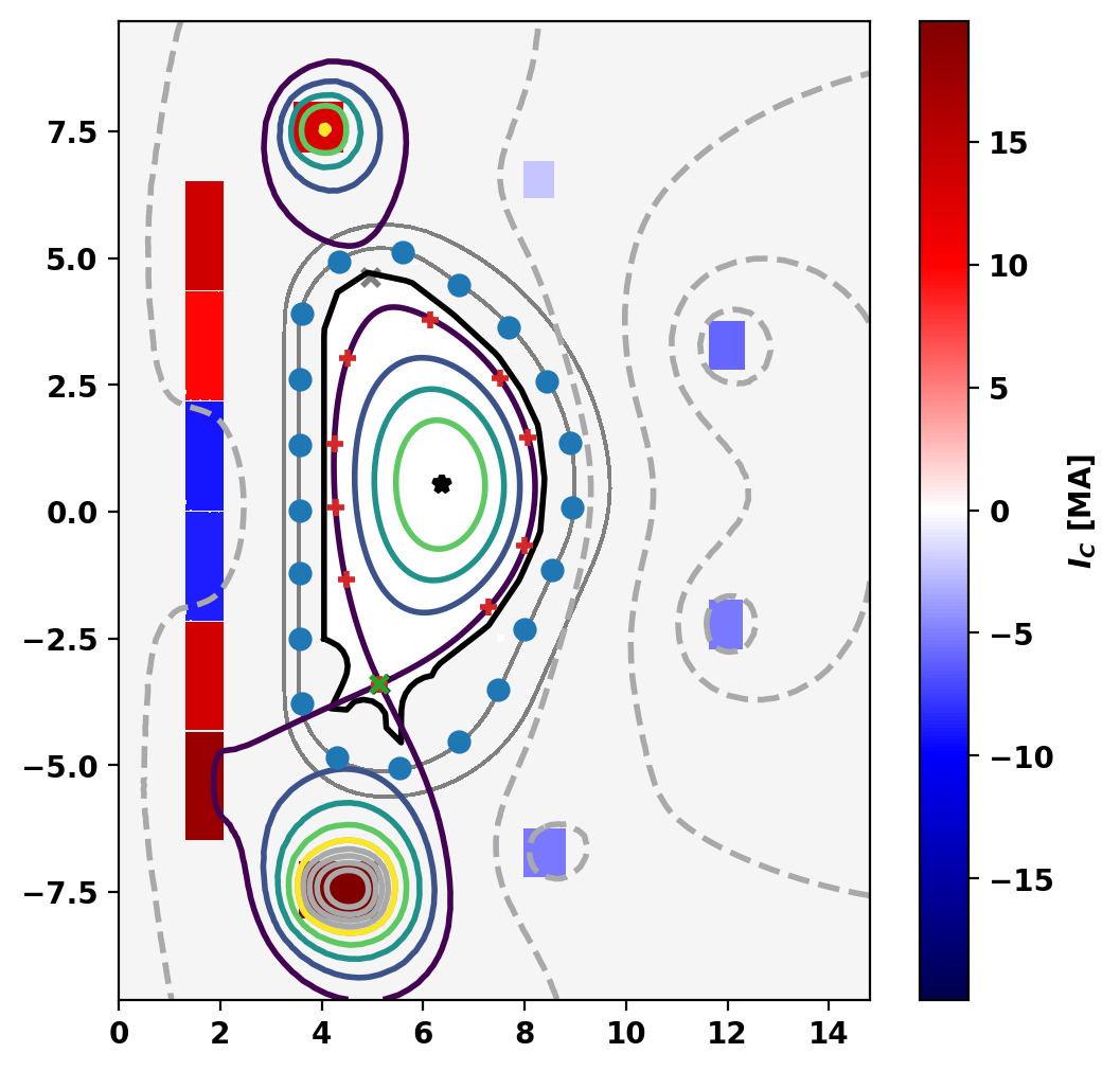
Print equilibrium information and coil currents

As above we use print_info() and get_coil_currents() to display information on the final equilibrium.

mygs.print_info()
 
print()
print("Coil Currents [MA]:")
coil_currents, _ = mygs.get_coil_currents()
for key, current in coil_currents.items():
    print('  {0:10} {1:10.2F}'.format(key+":",current/1.E6))

Equilibrium Statistics:
  Topology                =   Diverted
  Toroidal Current [A]    =    1.5733E+07
  Current Centroid [m]    =    6.216  0.517
  Magnetic Axis [m]       =    6.377  0.522
  Elongation              =    1.889 (U:  1.768, L:  2.009)
  Triangularity           =    0.472 (U:  0.405, L:  0.539)
  Plasma Volume [m^3]     =   822.871
  q_0, q_95               =    0.840  2.757
  Plasma Pressure [Pa]    =   Axis:  6.9104E+05, Peak:  6.9104E+05
  Stored Energy [J]       =    2.7467E+08
  <Beta_pol> [%]          =   47.5304
  <Beta_tor> [%]          =    2.0102
  <Beta_n>   [%]          =    1.3337
  Diamagnetic flux [Wb]   =    1.4520E+00
  Toroidal flux [Wb]      =    1.2189E+02
  l_i                     =    1.1327

Coil Currents [MA]:
  CS3U:           13.64
  CS2U:            9.89
  CS1U:           -9.12
  CS1L:           -8.94
  CS2L:           13.36
  CS3L:           17.97
  PF1:            12.95
  PF2:            -2.23
  PF3:            -5.92
  PF4:            -5.35
  PF5:            -4.97
  PF6:            19.56
  VS:              0.15

Plot final reconstructed equilibrium

fig, ax = plt.subplots(1,1)
mygs.plot_machine(fig,ax,coil_colormap='seismic',coil_scale=1.E-6,coil_clabel=r'$I_C$ [MA]',coil_symmap=True)
mygs.plot_psi(fig,ax,plasma_nlevels=5,vacuum_nlevels=5)
mygs.plot_psi(fig,ax,psi_target,plasma_levels=[1.0,],plasma_color='red',vacuum_nlevels=0,plasma_linestyles='dashed')