In this example we show how to compute simple equilibria in HBT-EP:
- The "inverse" case where we have a desired shape, plasma current and pressure, but the required coil currents are unkown
- The "forward" case where we have already have coil currents, plasma current, and known position for the desired equilibrium
This example utilizes the mesh built in TokaMaker Meshing Example: Building a mesh for HBT-EP.
- Note
- Running this example requires the h5py python package, which is installable using
pipor other standard methods.
Load TokaMaker library
To load the TokaMaker python module we need to tell python where to the module is located. This can be done either through the PYTHONPATH environment variable or using within a script using sys.path.append() as below, where we look for the environement variable OFT_ROOTPATH to provide the path to where the OpenFUSIONToolkit is installed (/Applications/OFT on macOS).
For meshing we will use the gs_Domain() class to build a 2D triangular grid suitable for Grad-Shafranov equilibria. This class uses the triangle code through a python wrapper.
Compute equilibria
Initialize TokaMaker object
We now create a OFT_env instance for execution using two threads and a TokaMaker instance to use for equilibrium calculations. Note at present only a single TokaMaker instance can be used per python kernel, so this command should only be called once in a given Jupyter notebook or python script. In the future this restriction may be relaxed.
#----------------------------------------------
Open FUSION Toolkit Initialized
Development branch:   v1_beta6
Revision id:          681e857
Parallelization Info:
  # of MPI tasks      =    1
  # of NUMA nodes     =    1
  # of OpenMP threads =    2
Fortran input file    = /var/folders/52/n5qxh27n4w19qxzqygz2btbw0000gn/T/oft_64655/oftpyin
XML input file        = none
Integer Precisions    =    4   8
Float Precisions      =    4   8  16
Complex Precisions    =    4   8
LA backend            = native
#----------------------------------------------
Load mesh into TokaMaker
Now we load the mesh generated in TokaMaker Meshing Example: Building a mesh for HBT-EP using load_gs_mesh() and setup_mesh(). Then we use setup_regions() to define the different region types. Finally, we call setup() to setup the required solver objects. During this call we can specify the desired element order (min=2, max=4) and the toroidal field through F0 = B0*R0, where B0 is the toroidal field at a reference location R0.
**** Loading OFT surface mesh

**** Generating surface grid level  1
  Generating boundary domain linkage
  Mesh statistics:
    Area         =  3.278E+00
    # of points  =    3736
    # of edges   =   11087
    # of cells   =    7352
    # of boundary points =     118
    # of boundary edges  =     118
    # of boundary cells  =     118
  Resolution statistics:
    hmin =  1.959E-04
    hrms =  3.418E-02
    hmax =  9.532E-02
  Surface grounded at vertex     804


**** Creating Lagrange FE space
  Order  =    2
  Minlev =   -1

 Computing flux BC matrix
 Inverting real matrix
   Time =    1.4220000000000001E-003
Define hard limits on coil currents
Hard limits on coil currents can be set using set_coil_bounds(). For HBT-EP, a limit of 20 kA/turn is set for the OH with 15 kA/turn for the VF and SH.
Bounds are specified using a dictionary of 2 element lists, containing the minimum and maximum bound, where the dictionary key corresponds to the coil names, which are available in mygs.coil_sets
Compute Inverse Equilibrium
Define global quantities and targets
For the inverse case we define a target for the plasma current (Ip) and the ratio of the contribtions of \( F*F' \) and \( P' \) to \( I_p \), which can be considered a proxy for \( \beta_p \).
- Note
- These constraints can be considered "hard" constraints, where they will be matched to good tolerance as long as the calculation converges.
Define shape targets
As HBT-EP has only a few coil sets there is limited shaping that is available. For the first case we just generate a standard circular plasma at a fixed location using isoflux points to set the rough radial and vertical bounds of the LCFS.
- Note
- These constraints can be considered "soft" constraints, where the calculation attempts to minimize error in satisfying these constraints subject to other constraints and regularization.
Define coil regularization matrix
In general, for a given coil set a given plasma shape cannot be exactly reproduced, which generally yields large amplitude coil currents if no constraint on the coil currents is applied. As a result, it is useful to include regularization terms for the coils to balance minimization of the shape error with the amplitude of current in the coils. In TokaMaker these regularization terms have the general form, where each term corresponds to a set of coil coefficients, target value, and weight. The coil_reg_term() method is provided to aid in defining these terms.
Here we use the identity as the regularization matrix:
- A target of 0 A and a modest weight for the
VFcoil - A target of -8 kA and a high weight for the
OHcoil - A target of 0 A and a high weight for the
SHcoil
The first regularization term weakly penalizes current in the VF coil to prevent large currents. While this is not strictly required in a simple case like HBT-EP it is generally necessary in configurations with more coils and higher shaping.
The second and third terms use high weights to force (approximately) the current in the OH and SH coils to -8 kA and 0 kA respectively.
Define flux functions
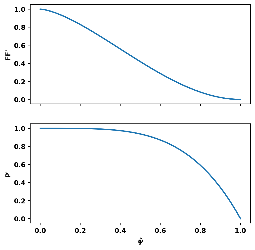
Although TokaMaker has a "default" profile for the F*F' and P' terms this should almost never be used and one should instead choose an appropriate flux function for their application. In this case we use an L-mode-like profile of the form \(((1-\hat{\psi})^{\alpha})^{\gamma}\), using create_power_flux_fun(), where \(\alpha\) and \(\gamma\) are set differently for F*F' and P' to provide peaked and broad profiles respectively. Within TokaMaker this profile is represented as a piecewise linear function, which can be set up using the dictionary approach shown below.
Compute equilibrium
We can now compute a free-boundary equilibrium using these constraints. Note that before running a calculation for the first time we must initialize the flux function \(\psi\), which can be done using init_psi(). This subroutine initializes the flux using the specified Ip_target from above, which is evenly distributed over the entire plasma region or only with a boundary defined using a center point (R,Z), minor radius (a), and elongation and triangularity. Coil currents are also initialized at this point using the constraints above and this uniform plasma current initialization.
solve() is then called to compute a self-consitent Grad-Shafranov equilibrium. If the result variable (err_flag) is zero then the solution has converged to the desired tolerance ( \(10^{-6}\) by default).
Starting non-linear GS solver
     1  1.9399E-02  3.1501E-01  3.0188E-04  9.3857E-01 -1.7715E-05 -0.0000E+00
     2  2.0101E-02  3.2139E-01  8.0636E-05  9.3962E-01 -1.6011E-05 -0.0000E+00
     3  2.0301E-02  3.2316E-01  2.2287E-05  9.3989E-01 -2.6169E-05 -0.0000E+00
     4  2.0365E-02  3.2372E-01  6.5134E-06  9.3998E-01 -3.1799E-05 -0.0000E+00
     5  2.0387E-02  3.2390E-01  1.9972E-06  9.4000E-01 -3.7284E-05 -0.0000E+00
     6  2.0394E-02  3.2396E-01  6.3248E-07  9.4001E-01 -4.2616E-05 -0.0000E+00
 Timing:   3.6635000025853515E-002
   Source:     1.7673000053036958E-002
   Solve:      1.1245999950915575E-002
   Boundary:   1.1719999602064490E-003
   Other:      6.5440000616945326E-003
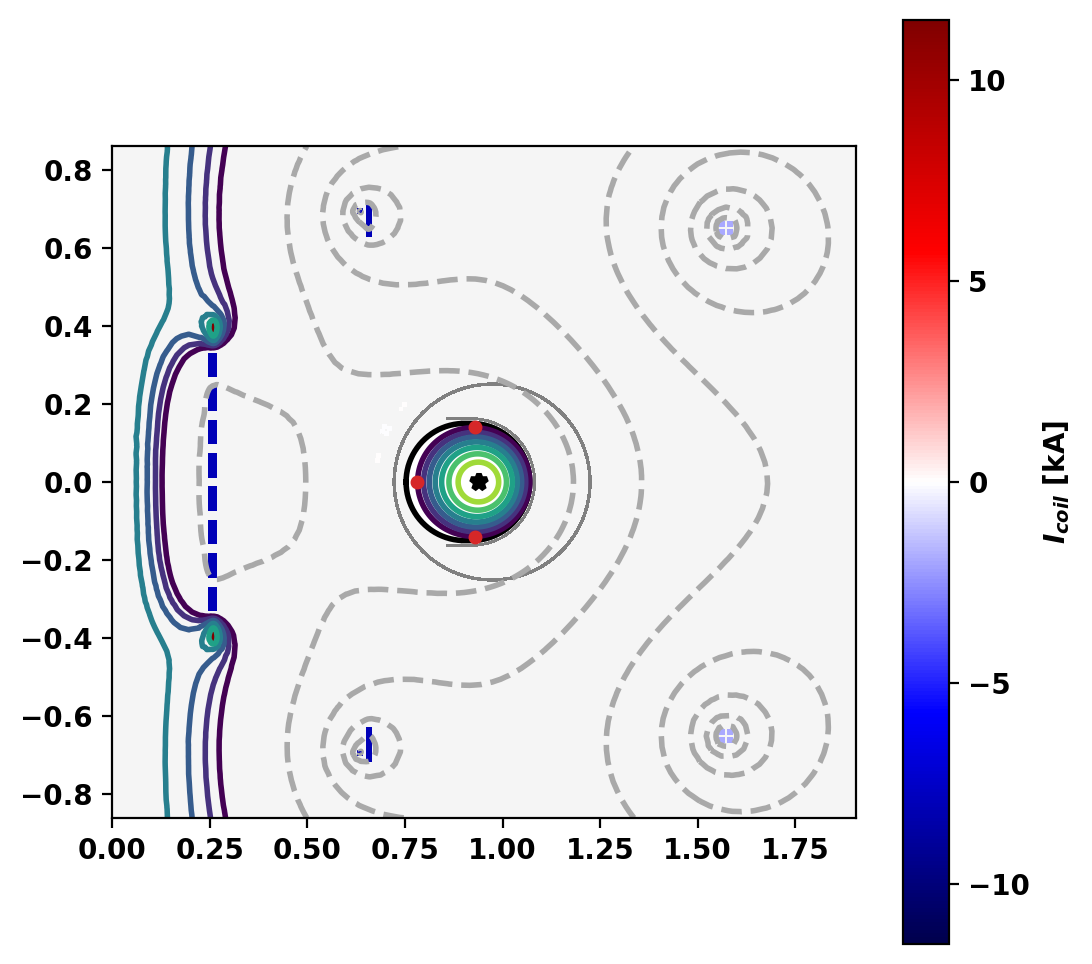
Plot equilibrium
Flux surfaces of the computed equilibrium can be plotted using the plot_psi() method. The additional plotting methods plot_machine() and plot_constraints() are also used to show context and other information. Each method has a large number of optional arguments for formatting and other options.
Print equilibrium information and coil currents
Basic parameters can be displayed using the print_info() method. For access to these quantities as variables instead the get_stats() can be used.
The final coil currents can also be retrieved using the get_coil_currents() method, which are all within the approximate coil limits imposed above.
Equilibrium Statistics:
  Topology                =   Limited
  Toroidal Current [A]    =    1.1928E+04
  Current Centroid [m]    =    0.933 -0.000
  Magnetic Axis [m]       =    0.940 -0.000
  Elongation              =    0.968 (U:  0.968, L:  0.968)
  Triangularity           =    0.003 (U: -0.003, L:  0.010)
  Plasma Volume [m^3]     =    0.365
  q_0, q_95               =    2.227  2.981
  Plasma Pressure [Pa]    =   Axis:  2.8217E+02, Peak:  2.8217E+02
  Stored Energy [J]       =    6.1610E+01
  <Beta_pol> [%]          =   99.1571
  <Beta_tor> [%]          =    0.2526
  <Beta_n>   [%]          =    1.0171
  Diamagnetic flux [Wb]   =    3.6725E-07
  Toroidal flux [Wb]      =    2.1126E-02
  l_i                     =    0.7131

Coil Currents [kA]:
  OH:             -8.00
  VF:             -1.92
  SH:              0.00
Compute forward equilibrium with shaping
Update global quantities and targets
For the forward case we re-define a target for the plasma current (Ip) and swap the Ip_ratio target for an R0 target, which constrains the location of the magnetic axis.
We also remove the isoflux targets so that the coil currents will remained fixed during the solve.
Set coil currents explicitly
Here we update the coil currents, which were retrieved above, to put current in the shaping coil (SH). Additionally, we slightly adjust current in the VF to produce a plasma with reasonable \(\beta_p\). Values are updated by passing an updated array to set_coil_currents().
Solve for updated equilibrium
As this solve is somewhat more challenging we increase the maximum number of solver iterations using the settings object and update_settings().
Starting non-linear GS solver
     1  1.8362E-01  2.7213E-01  1.7497E-03  9.4000E-01  4.9598E-04  0.0000E+00
     2  3.3455E-01  2.6822E-01  3.5215E-04  9.3998E-01  1.1622E-03  0.0000E+00
     3  4.8616E-01  2.5806E-01  7.2479E-05  9.3996E-01  1.8002E-03  0.0000E+00
     4  5.8778E-01  2.4105E-01  1.7202E-05  9.3996E-01  2.4049E-03  0.0000E+00
     5  6.5441E-01  2.2767E-01  7.0824E-06  9.3996E-01  2.9794E-03  0.0000E+00
     6  6.9651E-01  2.1901E-01  4.9237E-06  9.3996E-01  3.5262E-03  0.0000E+00
     7  7.2257E-01  2.1389E-01  4.0626E-06  9.3996E-01  4.0498E-03  0.0000E+00
     8  7.3765E-01  2.1135E-01  3.5890E-06  9.3996E-01  4.5508E-03  0.0000E+00
     9  7.4649E-01  2.1023E-01  3.3133E-06  9.3996E-01  5.0314E-03  0.0000E+00
    10  7.5152E-01  2.1000E-01  3.1344E-06  9.3997E-01  5.4934E-03  0.0000E+00
    11  7.5418E-01  2.1031E-01  3.0002E-06  9.3997E-01  5.9389E-03  0.0000E+00
    12  7.5538E-01  2.1094E-01  2.8838E-06  9.3997E-01  6.3688E-03  0.0000E+00
    13  7.5569E-01  2.1177E-01  2.7785E-06  9.3997E-01  6.7834E-03  0.0000E+00
    14  7.5547E-01  2.1270E-01  2.6782E-06  9.3997E-01  7.1832E-03  0.0000E+00
    15  7.5491E-01  2.1368E-01  2.5841E-06  9.3997E-01  7.5685E-03  0.0000E+00
    16  7.5414E-01  2.1469E-01  2.4949E-06  9.3997E-01  7.9400E-03  0.0000E+00
    17  7.5327E-01  2.1569E-01  2.4103E-06  9.3998E-01  8.2983E-03  0.0000E+00
    18  7.5238E-01  2.1668E-01  2.3286E-06  9.3998E-01  8.6438E-03  0.0000E+00
    19  7.5147E-01  2.1765E-01  2.2512E-06  9.3998E-01  8.9772E-03  0.0000E+00
    20  7.5057E-01  2.1858E-01  2.1755E-06  9.3998E-01  9.2989E-03  0.0000E+00
    21  7.4969E-01  2.1949E-01  2.1014E-06  9.3998E-01  9.6095E-03  0.0000E+00
    22  7.4882E-01  2.2037E-01  2.0312E-06  9.3998E-01  9.9091E-03  0.0000E+00
    23  7.4799E-01  2.2122E-01  1.9622E-06  9.3998E-01  1.0198E-02  0.0000E+00
    24  7.4713E-01  2.2206E-01  1.8941E-06  9.3998E-01  1.0477E-02  0.0000E+00
    25  7.4623E-01  2.2288E-01  1.8267E-06  9.3998E-01  1.0746E-02  0.0000E+00
    26  7.4532E-01  2.2369E-01  1.7618E-06  9.3998E-01  1.1005E-02  0.0000E+00
    27  7.4441E-01  2.2447E-01  1.7007E-06  9.3998E-01  1.1255E-02  0.0000E+00
    28  7.4350E-01  2.2524E-01  1.6392E-06  9.3998E-01  1.1485E-02  0.0000E+00
    29  7.4204E-01  2.2614E-01  1.5790E-06  9.3998E-01  1.1715E-02  0.0000E+00
    30  7.4143E-01  2.2677E-01  1.5292E-06  9.3999E-01  1.1936E-02  0.0000E+00
    31  7.4073E-01  2.2742E-01  1.4774E-06  9.3999E-01  1.2149E-02  0.0000E+00
    32  7.4002E-01  2.2807E-01  1.4267E-06  9.3999E-01  1.2355E-02  0.0000E+00
    33  7.3931E-01  2.2869E-01  1.3767E-06  9.3999E-01  1.2554E-02  0.0000E+00
    34  7.3863E-01  2.2929E-01  1.3276E-06  9.3999E-01  1.2745E-02  0.0000E+00
    35  7.3796E-01  2.2988E-01  1.2799E-06  9.3999E-01  1.2929E-02  0.0000E+00
    36  7.3731E-01  2.3044E-01  1.2337E-06  9.3999E-01  1.3107E-02  0.0000E+00
    37  7.3670E-01  2.3098E-01  1.1887E-06  9.3999E-01  1.3278E-02  0.0000E+00
    38  7.3610E-01  2.3150E-01  1.1455E-06  9.3999E-01  1.3442E-02  0.0000E+00
    39  7.3551E-01  2.3201E-01  1.1038E-06  9.3999E-01  1.3601E-02  0.0000E+00
    40  7.3494E-01  2.3250E-01  1.0636E-06  9.3999E-01  1.3753E-02  0.0000E+00
    41  7.3438E-01  2.3297E-01  1.0245E-06  9.3999E-01  1.3900E-02  0.0000E+00
    42  7.3385E-01  2.3342E-01  9.8647E-07  9.3999E-01  1.4041E-02  0.0000E+00
 Timing:  0.21114999998826534
   Source:     9.7579999652225524E-002
   Solve:      7.4561000103130937E-002
   Boundary:   7.5180003186687827E-003
   Other:      3.1490999914240092E-002
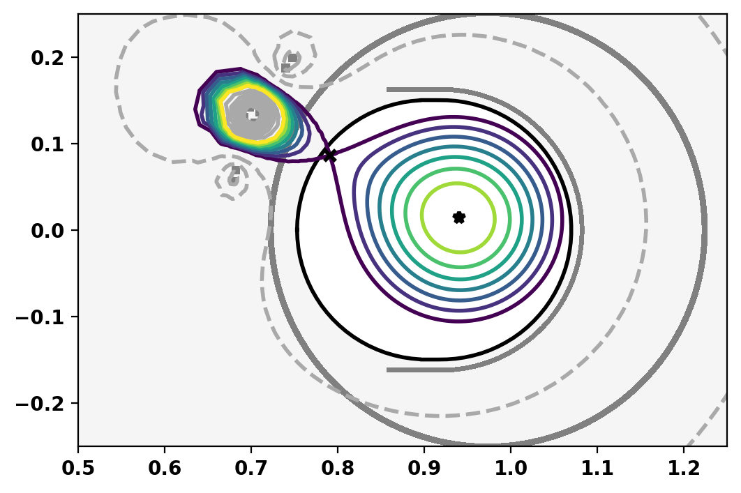
Plot equilibrium
Print equilibrium information and coil currents
Equilibrium Statistics:
  Topology                =   Diverted
  Toroidal Current [A]    =    1.1921E+04
  Current Centroid [m]    =    0.936  0.015
  Magnetic Axis [m]       =    0.940  0.014
  Elongation              =    0.879 (U:  0.866, L:  0.893)
  Triangularity           =   -0.086 (U: -0.062, L: -0.109)
  Plasma Volume [m^3]     =    0.281
  q_0, q_95               =    1.159  2.305
  Plasma Pressure [Pa]    =   Axis:  2.4719E+02, Peak:  2.4719E+02
  Stored Energy [J]       =    3.7206E+01
  <Beta_pol> [%]          =   63.1048
  <Beta_tor> [%]          =    0.1976
  <Beta_n>   [%]          =    0.7462
  Diamagnetic flux [Wb]   =    1.0665E-05
  Toroidal flux [Wb]      =    1.6102E-02
  l_i                     =    0.9748

Coil Currents [kA]:
  OH:             -8.00
  VF:             -1.65
  SH:             -7.00