In this example we demonstrate:
- How to create a sequence of positive triangularity CUTE equilibrium using a inverse solves
- How to compute linear and nonlinear growth rates for each case and plot the results
This example utilizes the mesh built in TokaMaker Meshing Example: Building a mesh for CUTE.
- Note
- Running this example requires the h5py python package, which is installable using
pipor other standard methods.
Load TokaMaker library
To load the TokaMaker python module we need to tell python where to the module is located. This can be done either through the PYTHONPATH environment variable or using within a script using sys.path.append() as below, where we look for the environement variable OFT_ROOTPATH to provide the path to where the OpenFUSIONToolkit is installed (/Applications/OFT on macOS).
Setup calculation
Initialize TokaMaker object
We now create a OFT_env instance for execution using two threads and a TokaMaker instance to use for equilibrium calculations. Note at present only a single TokaMaker instance can be used per python kernel, so this command should only be called once in a given Jupyter notebook or python script. In the future this restriction may be relaxed.
#----------------------------------------------
Open FUSION Toolkit Initialized
Development branch:   v1_beta6
Revision id:          681e857
Parallelization Info:
  # of MPI tasks      =    1
  # of NUMA nodes     =    1
  # of OpenMP threads =    2
Fortran input file    = /var/folders/52/n5qxh27n4w19qxzqygz2btbw0000gn/T/oft_64576/oftpyin
XML input file        = none
Integer Precisions    =    4   8
Float Precisions      =    4   8  16
Complex Precisions    =    4   8
LA backend            = native
#----------------------------------------------
Load mesh into TokaMaker
Now we load the mesh generated in TokaMaker Meshing Example: Building a mesh for CUTE using load_gs_mesh() and setup_mesh. Then we use setup_regions(), passing the conductor and coil dictionaries for the mesh, to define the different region types. Finally, we call setup() to setup the required solver objects. During this call we can specify the desired element order (min=2, max=4) and the toroidal field through F0 = B0*R0, where B0 is the toroidal field at a reference location R0.
**** Loading OFT surface mesh

**** Generating surface grid level  1
  Generating boundary domain linkage
  Mesh statistics:
    Area         =  1.301E+00
    # of points  =    5796
    # of edges   =   17283
    # of cells   =   11488
    # of boundary points =     102
    # of boundary edges  =     102
    # of boundary cells  =     102
  Resolution statistics:
    hmin =  3.994E-03
    hrms =  1.721E-02
    hmax =  7.410E-02
  Surface grounded at vertex     761


**** Creating Lagrange FE space
  Order  =    2
  Minlev =   -1

 Computing flux BC matrix
 Inverting real matrix
   Time =    9.3199999999999999E-004
Define hard limits on coil currents
Hard limits on coil currents can be set using set_coil_bounds(). For CUTE, a limit of 1 kA per turn is assumed.
Bounds are specified using a dictionary of 2 element lists, containing the minimum and maximum bound, where the dictionary key corresponds to the coil names, which are available in mygs.coil_sets
Define coil regularization matrix
In general, for a given coil set a given plasma shape cannot be exactly reproduced, which generally yields large amplitude coil currents if no constraint on the coil currents is applied. As a result, it is useful to include regularization terms for the coils to balance minimization of the shape error with the amplitude of current in the coils. In TokaMaker these regularization terms have the general form, where each term corresponds to a set of coil coefficients, target value, and weight. The coil_reg_term() method is provided to aid in defining these terms.
Below we define two types of regularization targets:
- Targets that act to penalize up-down assymetry in up-down coil pairs, which are defined in the
coil_mirrorsdictionary. - Targets the act to penalize the amplitude of current in each coil.
In the later case this regularization acts to penalize the amplitude of current in each coil, acting to balance coil currents with error in the shape targets. Additionally, this target is also used to "disable" several coils by setting the weight on their targets high to strongly penalize non-zero current.
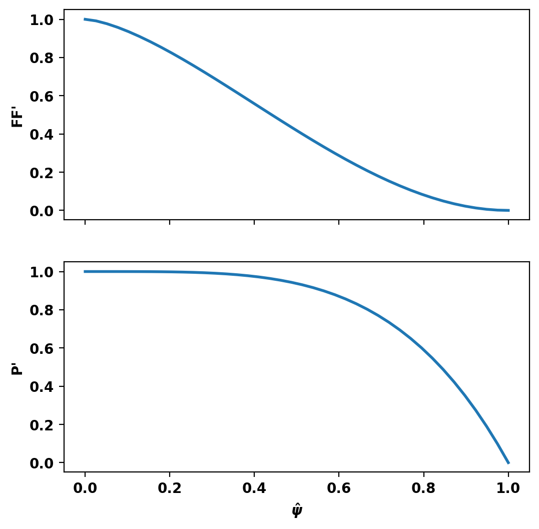
Define flux functions
Although TokaMaker has a "default" profile for the F*F' and P' terms this should almost never be used and one should instead choose an appropriate flux function for their application. In this case we use an L-mode-like profile of the form \(((1-\hat{\psi})^{\alpha})^{\gamma}\), using create_power_flux_fun(), where \(\alpha\) and \(\gamma\) are set differently for F*F' and P' to provide peaked and broad profiles respectively. Within TokaMaker this profile is represented as a piecewise linear function, which can be set up using the dictionary approach shown below.
Define global quantities and targets
For the Grad-Shafranov solve we define targets for the plasma current and the ratio the F*F' and P' contributions to the plasma current, which is approximately related to \(\beta_p\) as Ip_ratio = \(1/\beta_p - 1\). In the scan below we will vary Ip_ratio to match different target \(\beta\) values.
- Note
- These constraints can be considered "hard" constraints, where they will be matched to good tolerance as long as the calculation converges.
Define shape targets
In order to constrain the shape of the plasma we can utilize two types of constraints:
isofluxpoints, which are points we want to lie on the same flux surface (eg. the LCFS)saddlepoints, where we want the poloidal magnetic field to vanish (eg. X-points). While one can also use this constraint to enforce a magnetic axis location, instead set_targets() should be used with argumentsR0andV0.
- Note
- These constraints can be considered "soft" constraints, where the calculation attempts to minimize error in satisfying these constraints subject to other constraints and regularization.
Here we define a handful of isoflux points that we want to lie on the outboard side of the LCFS for the target equilibrium. Additionally, we define a two X-points and set them as saddle constraints. We also add the lower X-point to the list of isoflux points as we would like that to also lie on the LCFS as the active X-point.
Compute initial equilibrium
We can now compute a free-boundary equilibrium using these constraints and a starting \(\beta_{approx}\) of 20%. Note that before running a calculation for the first time we must initialize the flux function \(\psi\), which can be done using init_psi(). This subroutine initializes the flux using the specified Ip_target, which is evenly distributed over the entire plasma region or only with a boundary defined using a center point (R,Z), minor radius (a), and elongation and triangularity. Coil currents are also initialized at this point using the constraints above and this uniform plasma current initialization.
solve() is then called to compute a self-consitent Grad-Shafranov equilibrium. If the result variable (err_flag) is zero then the solution has converged to the desired tolerance ( \(10^{-6}\) by default).
Starting non-linear GS solver
     1  2.3289E+00  1.4875E+00  6.3391E-03  3.4320E-01  7.3704E-04 -0.0000E+00
     2  2.5451E+00  1.5358E+00  1.4525E-03  3.4134E-01  7.1572E-04 -0.0000E+00
     3  2.6170E+00  1.5572E+00  4.1092E-04  3.4050E-01  6.9276E-04 -0.0000E+00
     4  2.6494E+00  1.5676E+00  1.4801E-04  3.4011E-01  6.7451E-04 -0.0000E+00
     5  2.6649E+00  1.5728E+00  6.2491E-05  3.3992E-01  6.6017E-04 -0.0000E+00
     6  2.6725E+00  1.5753E+00  2.8539E-05  3.3983E-01  6.4897E-04 -0.0000E+00
     7  2.6763E+00  1.5765E+00  1.3565E-05  3.3979E-01  6.4034E-04 -0.0000E+00
     8  2.6782E+00  1.5771E+00  6.6502E-06  3.3977E-01  6.3376E-04 -0.0000E+00
     9  2.6792E+00  1.5775E+00  3.4125E-06  3.3976E-01  6.2878E-04 -0.0000E+00
    10  2.6797E+00  1.5776E+00  1.8961E-06  3.3976E-01  6.2504E-04 -0.0000E+00
    11  2.6800E+00  1.5777E+00  1.1724E-06  3.3976E-01  6.2225E-04 -0.0000E+00
    12  2.6802E+00  1.5777E+00  7.9698E-07  3.3976E-01  6.2018E-04 -0.0000E+00
 Timing:  0.18066700000781566
   Source:     9.0711000026203692E-002
   Solve:      4.0235000022221357E-002
   Boundary:   4.1819999460130930E-003
   Other:      4.5539000013377517E-002
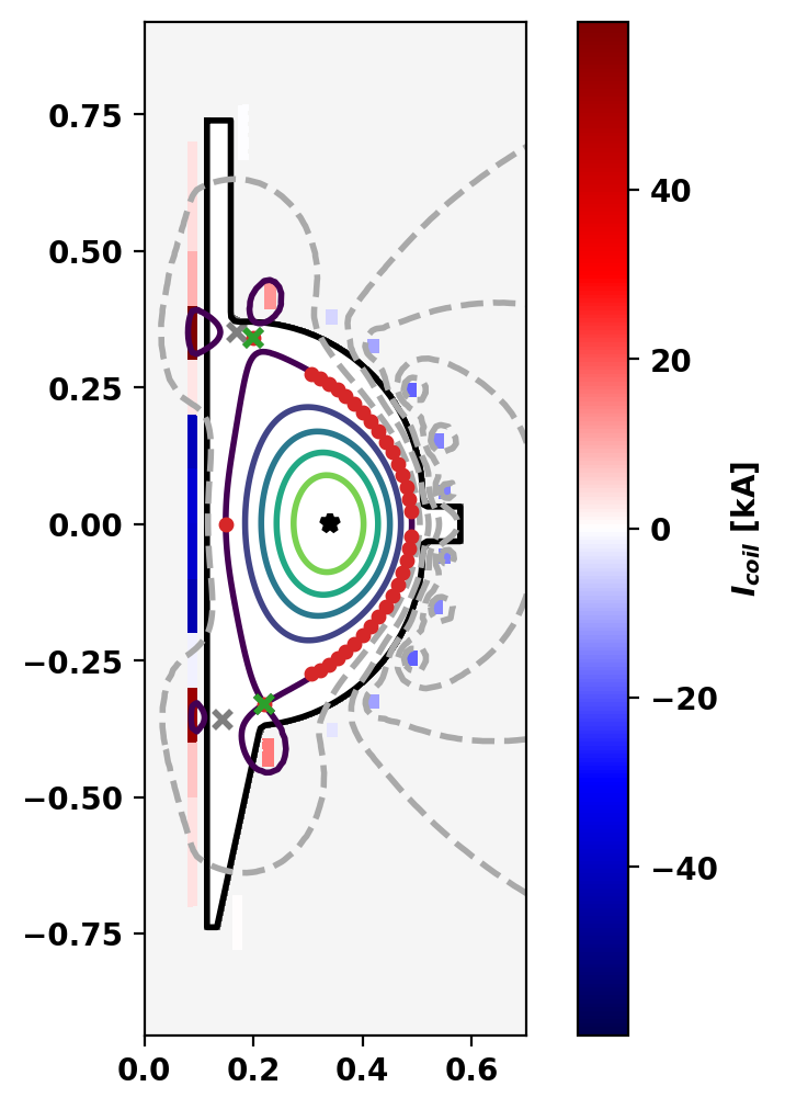
Plot initial equilibrium
Flux surfaces of the computed equilibrium can be plotted using the plot_psi() method. The additional plotting methods plot_machine() and plot_constraints() are also used to show context and other information. Each method has a large number of optional arguments for formatting and other options.
Run stability scan
Update settings
To reduce output we update settings to disable "performance monitoring" (eg. solver progress).
Compute linear stability as a function of \(\beta_p\)
Now we perform a scan of \(\beta_p\), computing the linear stability properties of the equilibrium at each point. We do this by looping over desired values of \(\beta_p\) and performing the following steps at each point:
- Compute the desired equilibrium by
- Set the shape constraints (needed as we remove them in step 3)
- Re-initialize \(\psi\) (needed as we evolve far from the initial equilibrium in step 3)
- Solve for the equilibrium, with a few iterations to converge the desired \(\beta_p\)
- Compute linear stability using eig_td()
- Save most unstable mode and growth rate
- Compute nonlinear evolution of a perturbed equilibrium
- Set the initial condition by adding a small contribution from the most unstable linear mode
- Remove saddle and isoflux constraints
- Setup the time-dependent solver
- Loop over 30 timesteps with a timestep determined by the linear growth rate, saving the equilibrium and vertical position at each time
Computing Beta_approx [%] 1.00
  Actual Beta_p = 1.00
Computing Beta_approx [%] 9.78
  Actual Beta_p = 9.74
Computing Beta_approx [%] 18.56
  Actual Beta_p = 18.78
Computing Beta_approx [%] 27.33
  Actual Beta_p = 27.60
Computing Beta_approx [%] 36.11
  Actual Beta_p = 35.98
Computing Beta_approx [%] 44.89
  Actual Beta_p = 44.80
Computing Beta_approx [%] 53.67
  Actual Beta_p = 53.84
Computing Beta_approx [%] 62.44
  Actual Beta_p = 62.37
Computing Beta_approx [%] 71.22
  Actual Beta_p = 71.11
Computing Beta_approx [%] 80.00
  Actual Beta_p = 79.93
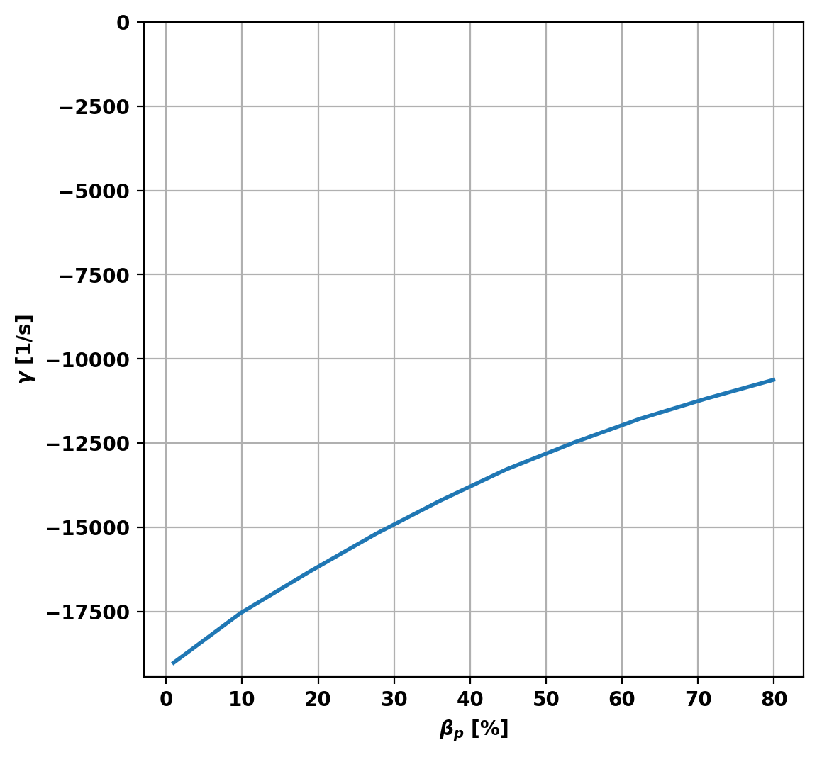
Plot growth rate trend
Once complete, we can plot the trend in the growth rate, which shows a decreasing growth rate for the vertical instability with increasing \(\beta_p\).
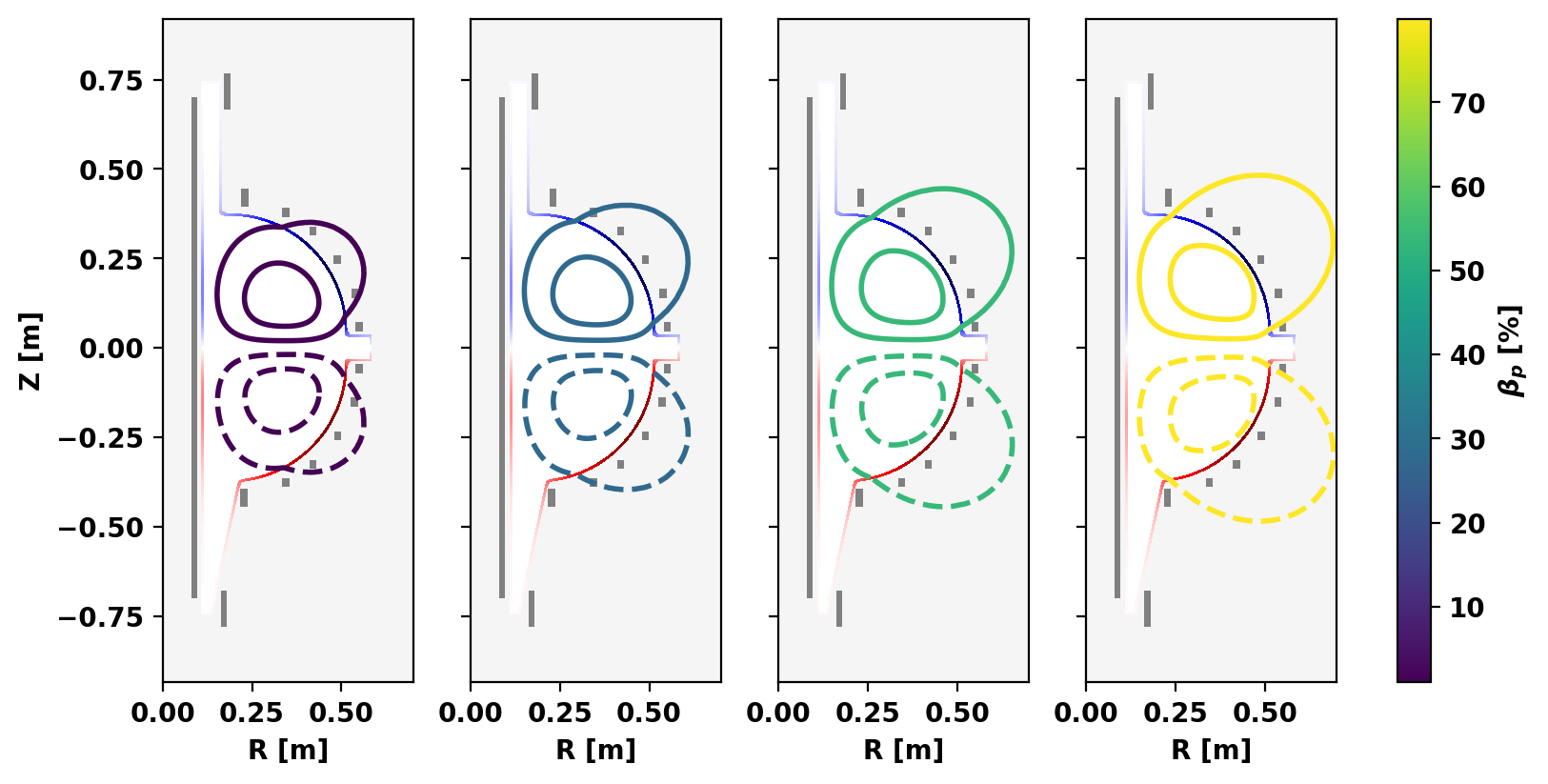
Plot linear eigenmodes
To better understand why this trend occurs, we can plot the linearly unstable mode structure as a function of \(\beta_p\). From this we can see that as \(\beta_p\) increases the mode structure shifts outboard and more of the perturbed flux (relative to the peak value) interacts with the wall. As the resistivity of the wall is what sets the timescale in a time-dependent Grad-Shafranov model, this explains the decrease in growth rate as as higher \(\beta_p\) more flux must move through the wall (via resisitive diffusion) for the same growth in amplitude.
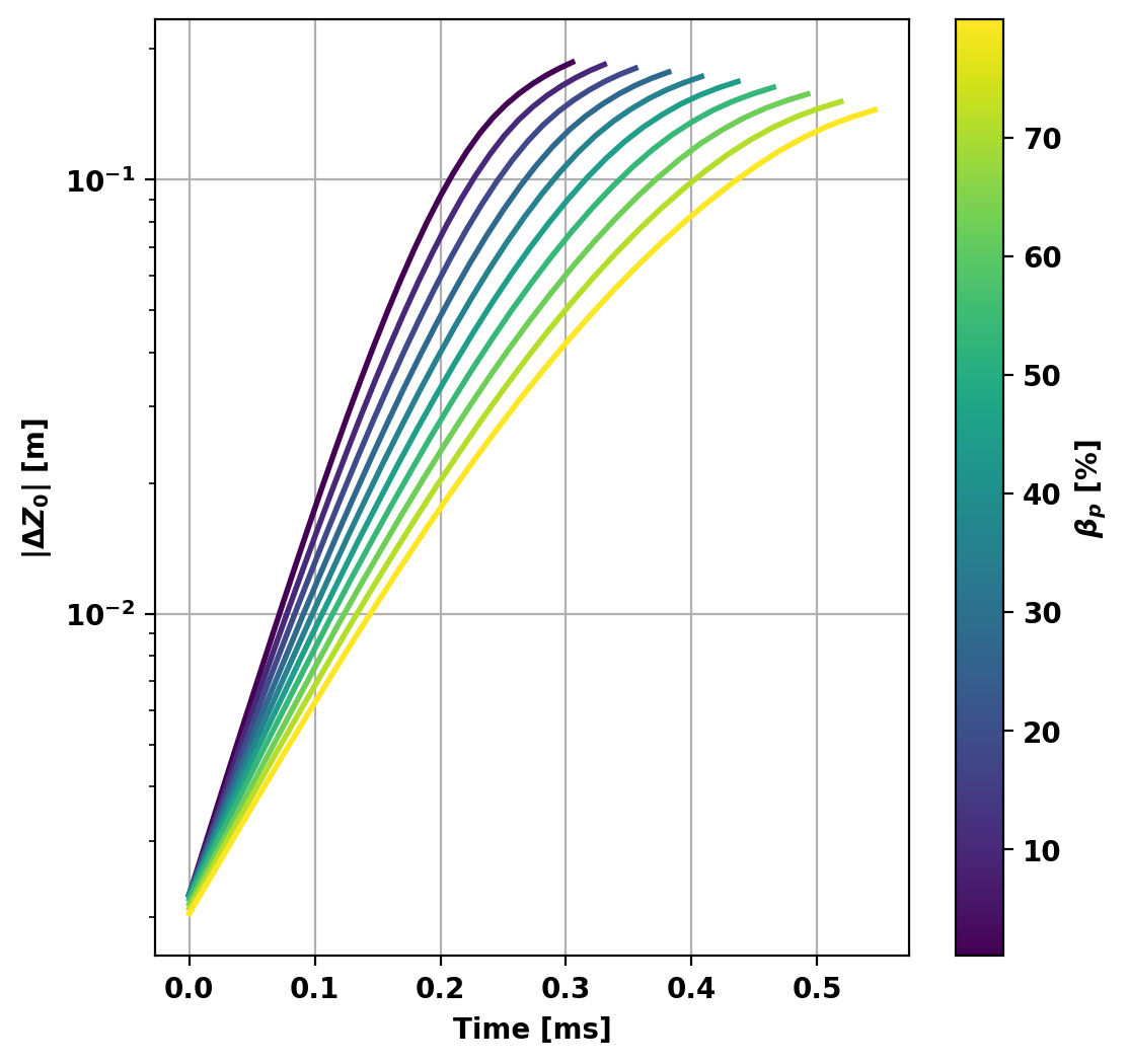
Plot nonlinear plasma evolution
We can also plot the evolution of the vertical position of the magnetic axis from the nonlinear evolution of each of the points in the \(\beta_p\) scan. This shows the same behavior as the linear study (as expected of course), where the growth rate (velocity of the vertical position) decreases with increasing \(\beta_p\). Additionally, clear linear (straight line on a log plot) and nonlinear phases are visible for each case.