 |
The Open FUSION Toolkit 26.9
An open-source framework for fusion and plasma science and engineering
|
Loading...
Searching...
No Matches
|
The Open FUSION Toolkit 26.9
An open-source framework for fusion and plasma science and engineering
|
Demonstrates the eqdsk module for reading standard GEQDSK (g-file) equilibrium files and Osborne p-files (kinetic profiles) without OMFIT or external dependencies.
What this notebook covers:
R_mag  = 1.7438 m
Z_mag  = -0.0053 m
Ip     = 1.2000 MA
B0     = 2.0243 T
R0     = 1.6796 m
psi_ax = 0.348276 Wb
psi_bd = 0.044025 Wb
COCOS  = 1
Grid   = 257 x 257
Every GEQDSKEquilibrium object exposes two introspection helpers:
Access any listed name as a normal attribute (eq.q_profile, eq.li, eq.geometry['kappa'], ...).
Available quantities (eq.keys):
  - Ip
  - R_mag
  - Z_mag
  - R_center
  - B_center
  - psi_axis
  - psi_boundary
  - cocos
  - fpol
  - pres
  - pprime
  - ffprim
  - qpsi
  - rhovn
  - psi_N
  - boundary_R
  - boundary_Z
  - limiter_R
  - limiter_Z
  - R_grid
  - Z_grid
  - psi_RZ
  - psi_N_RZ
  - q_profile
  - j_tor_averaged
  - j_tor_averaged_direct
  - j_tor_averaged_numerical
  - j_tor_over_R
  - geometry
  - averages
  - midplane
  - li
  - betas
  - contours

GEQDSKEquilibrium (COCOS 1, NW=257, NH=257, nlevels=257)
==============================================================================

Global scalars
--------------
  Ip                             Plasma current                                   [A]
                                   -> 1.20004e+06
  R_mag                          Magnetic axis R                                  [m]
                                   -> 1.74382
  Z_mag                          Magnetic axis Z                                  [m]
                                   -> -0.00531558
  R_center                       Reference geometric center R                     [m]
                                   -> 1.67955
  B_center                       Vacuum toroidal field at R_center                [T]
                                   -> 2.02435
  psi_axis                       Poloidal flux at magnetic axis                   [Wb]
                                   -> 0.348276
  psi_boundary                   Poloidal flux at LCFS                            [Wb]
                                   -> 0.0440249
  cocos                          COCOS convention index
                                   -> 1

1-D profiles (raw, on uniform psi_N from g-file)
------------------------------------------------
  fpol                           F = R * B_t                                      [T m]
                                   -> array (257,)
  pres                           Pressure                                         [Pa]
                                   -> array (257,)
  pprime                         dP/dpsi                                          [Pa/Wb]
                                   -> array (257,)
  ffprim                         F * dF/dpsi                                      [T^2 m^2/Wb]
                                   -> array (257,)
  qpsi                           Safety factor (from file)
                                   -> array (257,)
  rhovn                          Normalised toroidal flux
                                   -> array (257,)
  psi_N                          Normalised psi level grid
                                   -> array (257,)

Boundary and limiter
--------------------
  boundary_R                     LCFS R coordinates                               [m]
                                   -> array (257,)
  boundary_Z                     LCFS Z coordinates                               [m]
                                   -> array (257,)
  limiter_R                      Limiter R coordinates                            [m]
                                   -> array (405,)
  limiter_Z                      Limiter Z coordinates                            [m]
                                   -> array (405,)

2-D grids
---------
  R_grid                         1-D R grid                                       [m]
                                   -> array (257,)
  Z_grid                         1-D Z grid                                       [m]
                                   -> array (257,)
  psi_RZ                         Poloidal flux on (R,Z) grid                      [Wb]
                                   -> array (257, 257)
  psi_N_RZ                       Normalised flux on (R,Z) grid
                                   -> array (257, 257)

Derived 1-D profiles (lazy, flux-surface averaged)
--------------------------------------------------
  q_profile                      Safety factor from FSA
                                   -> (lazy; call describe(verbose=True) or access to compute)
  j_tor_averaged                 <Jt/R>/<1/R> (standard)                          [A/m^2]
                                   -> (lazy; call describe(verbose=True) or access to compute)
  j_tor_averaged_direct          <Jt> from GS                                     [A/m^2]
                                   -> (lazy; call describe(verbose=True) or access to compute)
  j_tor_averaged_numerical       <Jt> via curl(B)/mu0                             [A/m^2]
                                   -> (lazy; call describe(verbose=True) or access to compute)
  j_tor_over_R                   <Jt/R> from GS                                   [A/m^3]
                                   -> (lazy; call describe(verbose=True) or access to compute)

Derived containers (lazy, dicts of arrays)
------------------------------------------
  geometry                       R,Z,a,kappa,delta,vol,cxArea,perimeter,...       [dict]
                                   -> (lazy; call describe(verbose=True) or access to compute)
  averages                       All FSA quantities (R,1/R,Bp,Bt,vp,q,ip,...)     [dict]
                                   -> (lazy; call describe(verbose=True) or access to compute)
  midplane                       Outboard midplane R,Z,Br,Bz,Bp,Bt,Btot           [dict]
                                   -> (lazy; call describe(verbose=True) or access to compute)
  li                             Internal inductance li(1),li(2),li(3),...        [dict]
                                   -> (lazy; call describe(verbose=True) or access to compute)
  betas                          Plasma betas beta_t, beta_p, beta_n              [dict]
                                   -> (lazy; call describe(verbose=True) or access to compute)
  contours                       List of (N,2) flux-surface (R,Z) contours        [list]
                                   -> (lazy; call describe(verbose=True) or access to compute)
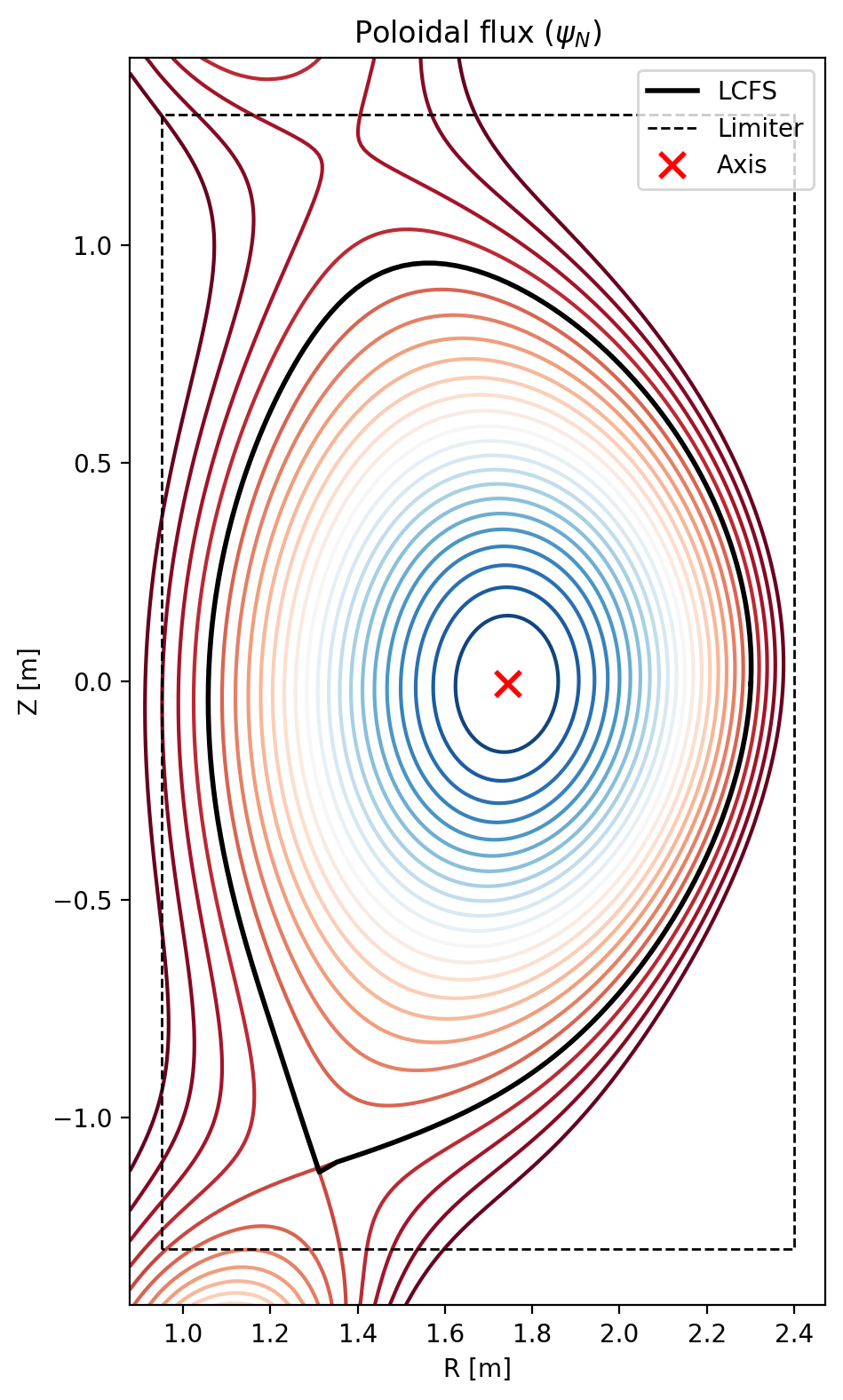
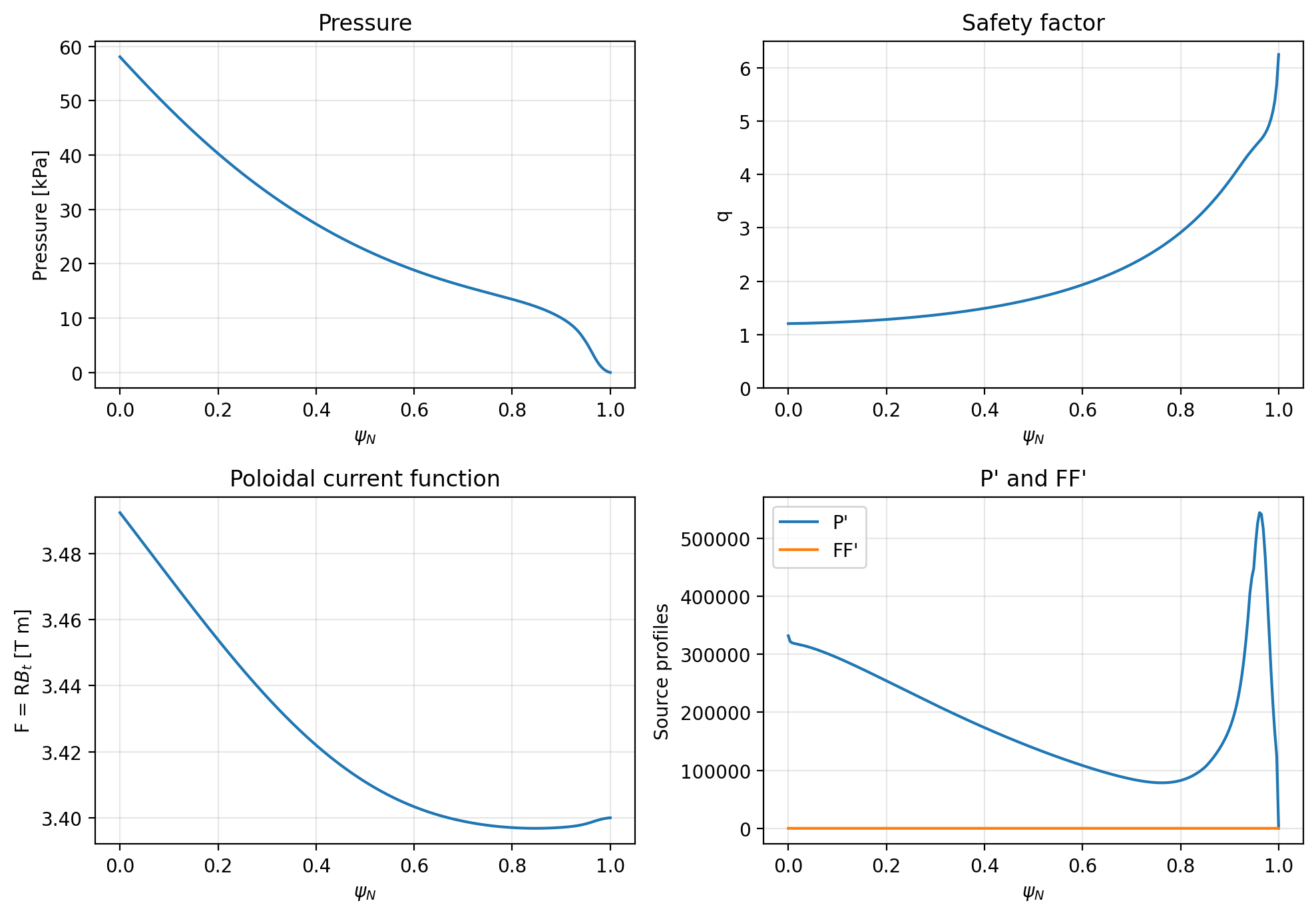
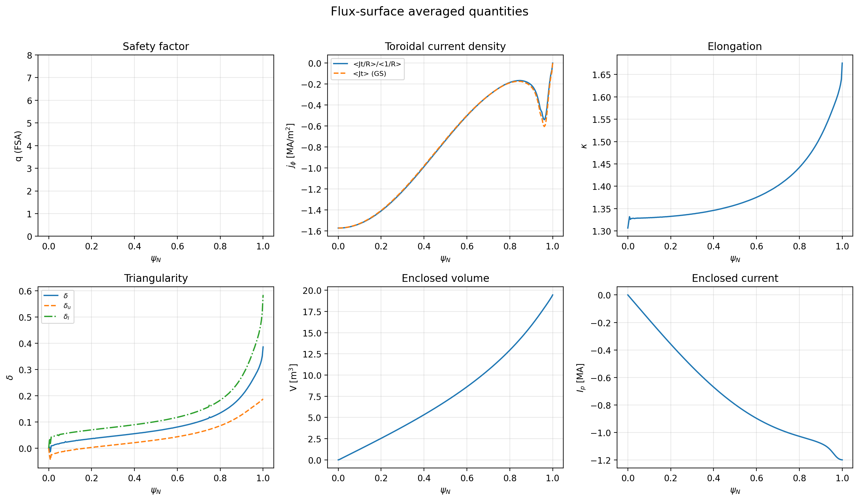
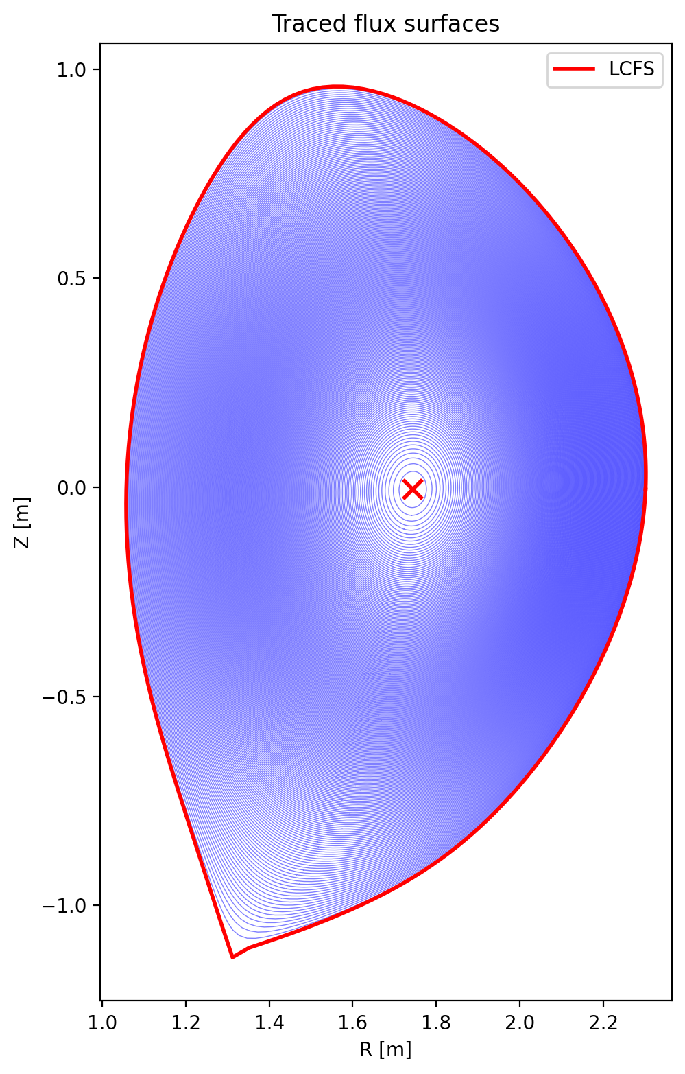
The GEQDSKEquilibrium class lazily traces flux-surface contours and computes averaged quantities on first access.
li(1) = 1.0660
li(3) = 0.8977
beta_t = 0.0130
beta_n = 1.3632
beta_p = 0.6430
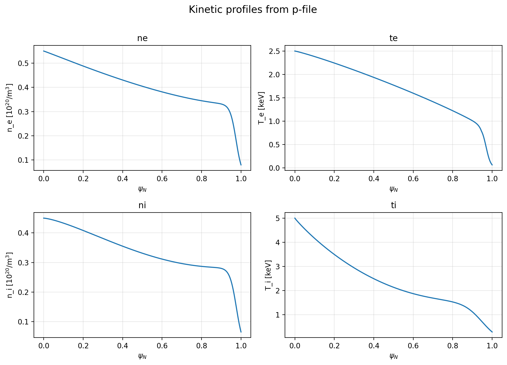
PFile(14 profiles: ne, te, ni, ti, nz1, ptot...)
Available profiles: ['ne', 'te', 'ni', 'ti', 'N Z A', 'nz1', 'ptot', 'omgpp', 'ommpp', 'omepp', 'omgeb', 'ommvb', 'omevb', 'er', 'omghb']
The PFile object has the same introspection pattern as the equilibrium:
PFile (15 entries)
==============================================================================

Kinetic profiles
----------------
  ne         Electron density                                 [10^20/m^3]
               -> len=514, range=[0.07984, 0.55]
  te         Electron temperature                             [KeV]
               -> len=514, range=[0.06425, 2.5]
  ni         Ion density                                      [10^20/m^3]
               -> len=514, range=[0.06508, 0.45]
  ti         Ion temperature                                  [KeV]
               -> len=514, range=[0.2881, 5]
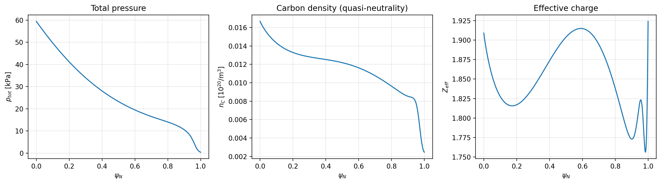
  ptot       Total pressure                                   [KPa]
               -> len=514, range=[0.3939, 59.41]

Rotation / Er
-------------
  omgpp      Diamagnetic term in the ExB rotation frequency   [kRad/s]
               -> len=514, range=[-13.02, -1.708]
  omgeb      ExB rotation frequency                           [kRad/s]
               -> len=514, range=[-13.02, -1.708]
  er         Radial electric field from force balance         [kV/m]
               -> len=514, range=[-0, 5.391]
  ommvb      Main ion VxB term of Er/RBp
               -> len=514, range=[4.828, 58.87]
  ommpp      Main ion pressure term of Er/RBp
               -> len=514, range=[-70.33, -6.65]
  omevb      Electron VxB term of Er/RBp
               -> len=514, range=[-107.5, -10.16]
  omepp      Electron pressure term of Er/RBp
               -> len=514, range=[6.408, 95.01]
  omghb      Hahm-Burrell ExB velocity shearing rate
               -> len=514, range=[-99.07, 66.03]

Impurity / beam
---------------
  nz1        Density of the 1st impurity species              [10^20/m^3]
               -> len=514, range=[0.002459, 0.01667]

Ion species (N, Z, A)
---------------------
  [0]  N=6  Z=6  A=12
  [1]  N=1  Z=1  A=2
  [2]  N=1  Z=1  A=2

Computable (not stored as profiles until you call these):
---------------------------------------------------------
  compute_pressure()           -> fills 'ptot'
  compute_quasineutrality()    -> fills 'nz1' from (ne - ni - nb)/Z_imp
  compute_zeff()               -> returns (psinorm, Zeff)
  compute_diamagnetic_rotations(psi)
                               -> fills omgpp, ommpp, omepp
  compute_rotation_decomposition(R, Bp, Bt, psi)
                               -> fills omgeb, ommvb, omevb, er, omghb
Original COCOS=1:  psi_axis = 0.348276
COCOS 11:                   psi_axis = 2.188282
Ratio = 6.283185  (expect 2*pi = 6.283185)
Ip:       1200039.50  ->  1200039.50  (err=0.00e+00)
psi_axis: 0.34827584  ->  0.34827584
psi_bdy:  0.04402488  ->  0.04402488
PSIRZ max err: 0.00e+00
FPOL max err:  0.00e+00
PRES max err:  0.00e+00
QPSI max err:  0.00e+00

Round-trip OK!
 1.17.0