 |
The Open FUSION Toolkit 26.9
An open-source framework for fusion and plasma science and engineering
|
Loading...
Searching...
No Matches
|
The Open FUSION Toolkit 26.9
An open-source framework for fusion and plasma science and engineering
|
In this example we demonstrate:
1) How to reproduce a DIII-D equilibrium using an inverse solve from EFIT by reading in inputs from a gEQDSK file. 2) How to reproduce a DIII-D equilibrium using an forward solve from EFIT by reading in inputs from a gEQDSK file. 3) How to compute linear growth rates and perform time-dependent simulation of a Vertical Displacement Event (VDE) using this equilibrium
This example utilizes the mesh built in TokaMaker Meshing Example: Building a mesh for DIII-D.
To load the TokaMaker python module we need to tell python where to the module is located. This can be done either through the PYTHONPATH environment variable or using within a script using sys.path.append() as below, where we look for the environement variable OFT_ROOTPATH to provide the path to where the OpenFUSIONToolkit is installed (/Applications/OFT on macOS).
We now create a OFT_env instance for execution using two threads and a TokaMaker instance to use for equilibrium calculations. Note at present only a single TokaMaker instance can be used per python kernel, so this command should only be called once in a given Jupyter notebook or python script. In the future this restriction may be relaxed.
#----------------------------------------------
             ____  ____________
            / __ \/ ____/_  __/
           / / / / /_    / /
          / /_/ / __/   / /
          \____/_/     /_/

Base release:        v1.0.0-beta7
Development branch:  release_26_06
Revision id:         978c4b9f

Parallelization Info:
  Not compiled with MPI
  # of OpenMP threads =    2

Linear Algebra backend: native

#----------------------------------------------
Now we load the mesh generated in TokaMaker Meshing Example: Building a mesh for DIII-D using load_gs_mesh() and setup_mesh. Then we use setup_regions(), passing the conductor and coil dictionaries for the mesh, to define the different region types. Finally, we call setup() to setup the required solver objects. During this call we can specify the desired element order (min=2, max=4) and the toroidal field through F0 = B0*R0, where B0 is the toroidal field at a reference location R0.
**** Loading OFT surface mesh

**** Generating surface grid level  1
  Generating boundary domain linkage
  Mesh statistics:
    Area         =  1.574E+01
    # of points  =    8911
    # of edges   =   26570
    # of cells   =   17660
    # of boundary points =     160
    # of boundary edges  =     160
    # of boundary cells  =     160
  Resolution statistics:
    hmin =  8.702E-04
    hrms =  4.833E-02
    hmax =  1.540E-01
  Surface grounded at vertex    1733


**** Creating Lagrange FE space
  Order  =    2
  Minlev =   -1

 Computing flux BC matrix
 Inverting real matrix
   Time =    2.0140000000000002E-003
Like many elongated equilibria, the equilibrium we seek to compute below is vertically unstable. In this case we use the F9A and F9B pair of poloidal field coils for vertical stability in order to help with convergence using the set_coil_vsc() method.
For the inverse case we define a target for the plasma current and the peak plasma pressure, which occurs on the magnetic axis.
In order to constrain the shape of the plasma we can utilize two types of constraints:
Here we use the contour defining the last closed flux surface as our isoflux constraint, and also set saddle targets to constrain the X-point locations.
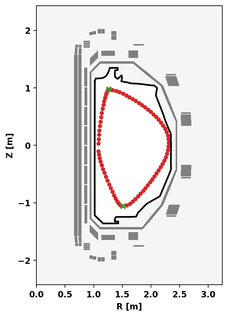
We aim to reproduce the gEQDSK equilibrium from EFIT with equivalent coil currents, so we use the current regularization matrix to constrain the TokaMaker coil currents to be close to the target values.
In this case, one regularization term is added for each coil with a single unit coefficient for that coil and target equal to the coil current from the input equilibrium. In this solve, the weights on the ECOILs are set high to prevent deviation from the target currents. Additionally, if a given poloidal field coil is found to have significant deviations from the target value, the weight on that coil can be increased, as is done below for F5A and F5B.
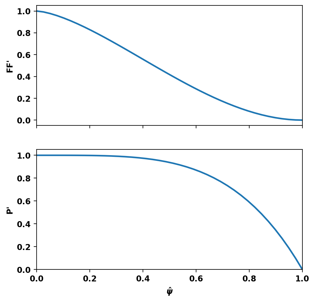
Although TokaMaker has a "default" profile for the \(FF'\) and \(P'\) terms this should almost never be used and one should instead choose an appropriate flux function for their application. In this case we use an L-mode-like profile of the form \(((1-\hat{\psi})^{\alpha})^{\gamma}\), using create_power_flux_fun(), where \(\alpha\) and \(\gamma\) are set differently for \(FF'\) and \(P'\) to provide peaked and broad profiles respectively. Within TokaMaker this profile is represented as a piecewise linear function, which can be set up using the dictionary approach shown below.
We can now compute a free-boundary equilibrium using these constraints. Note that before running a calculation for the first time we must initialize the flux function \(\psi\), which can be done using init_psi(). This subroutine initializes the flux using the specified Ip_target from above, which is evenly distributed over the entire plasma region or only with a boundary defined using a center point (R,Z), minor radius (a), and elongation and triangularity. Coil currents are also initialized at this point using the constraints above and this uniform plasma current initialization.
solve() is then called to compute a self-consitent Grad-Shafranov equilibrium. If the result variable (err_flag) is zero then the solution has converged to the desired tolerance ( \(10^{-6}\) by default).
Starting non-linear GS solver
     1  3.4341E+00  1.4377E-01  4.2224E-02  1.7476E+00 -5.0502E-02  1.4964E+03
     2  3.3961E+00  7.8292E-02  2.3591E-02  1.7391E+00 -3.7289E-02  1.1934E+03
     3  3.1612E+00  7.6150E-02  1.2127E-02  1.7341E+00 -2.5941E-02  9.3751E+02
     4  3.0316E+00  7.8379E-02  5.8972E-03  1.7314E+00 -1.7425E-02  7.7884E+02
     5  2.9723E+00  8.0153E-02  2.8864E-03  1.7299E+00 -1.1515E-02  6.9287E+02
     6  2.9418E+00  8.0960E-02  1.5765E-03  1.7291E+00 -7.5701E-03  6.4305E+02
     7  2.9259E+00  8.1364E-02  9.0898E-04  1.7288E+00 -5.0237E-03  6.1290E+02
     8  2.9177E+00  8.1572E-02  5.3988E-04  1.7285E+00 -3.3993E-03  5.9432E+02
     9  2.9135E+00  8.1682E-02  3.2650E-04  1.7284E+00 -2.3689E-03  5.8278E+02
    10  2.9113E+00  8.1738E-02  1.9983E-04  1.7284E+00 -1.7169E-03  5.7558E+02
    11  2.9101E+00  8.1768E-02  1.2332E-04  1.7283E+00 -1.3047E-03  5.7108E+02
    12  2.9096E+00  8.1783E-02  7.6547E-05  1.7283E+00 -1.0443E-03  5.6825E+02
    13  2.9093E+00  8.1791E-02  4.7722E-05  1.7283E+00 -8.7967E-04  5.6648E+02
    14  2.9092E+00  8.1795E-02  2.9849E-05  1.7283E+00 -7.7564E-04  5.6537E+02
    15  2.9091E+00  8.1797E-02  1.8717E-05  1.7283E+00 -7.0988E-04  5.6467E+02
    16  2.9091E+00  8.1798E-02  1.1759E-05  1.7283E+00 -6.6832E-04  5.6423E+02
    17  2.9091E+00  8.1798E-02  7.3977E-06  1.7283E+00 -6.4204E-04  5.6395E+02
    18  2.9090E+00  8.1798E-02  4.6592E-06  1.7283E+00 -6.2543E-04  5.6377E+02
    19  2.9090E+00  8.1798E-02  2.9371E-06  1.7283E+00 -6.1492E-04  5.6366E+02
    20  2.9090E+00  8.1798E-02  1.8527E-06  1.7283E+00 -6.0828E-04  5.6359E+02
    21  2.9090E+00  8.1798E-02  1.1693E-06  1.7283E+00 -6.0408E-04  5.6355E+02
    22  2.9090E+00  8.1798E-02  7.3832E-07  1.7283E+00 -6.0143E-04  5.6352E+02
 Timing:  0.24931199999991804
   Source:    0.11960299994098023
   Solve:      6.3162999926134944E-002
   Boundary:   5.2709999727085233E-003
   Other:      6.1275000160094351E-002
Flux surfaces of the computed equilibrium can be plotted using the plot_psi() method. The additional plotting methods plot_machine() and plot_constraints() are also used to show context and other information. Each method has a large number of optional arguments for formatting and other options.
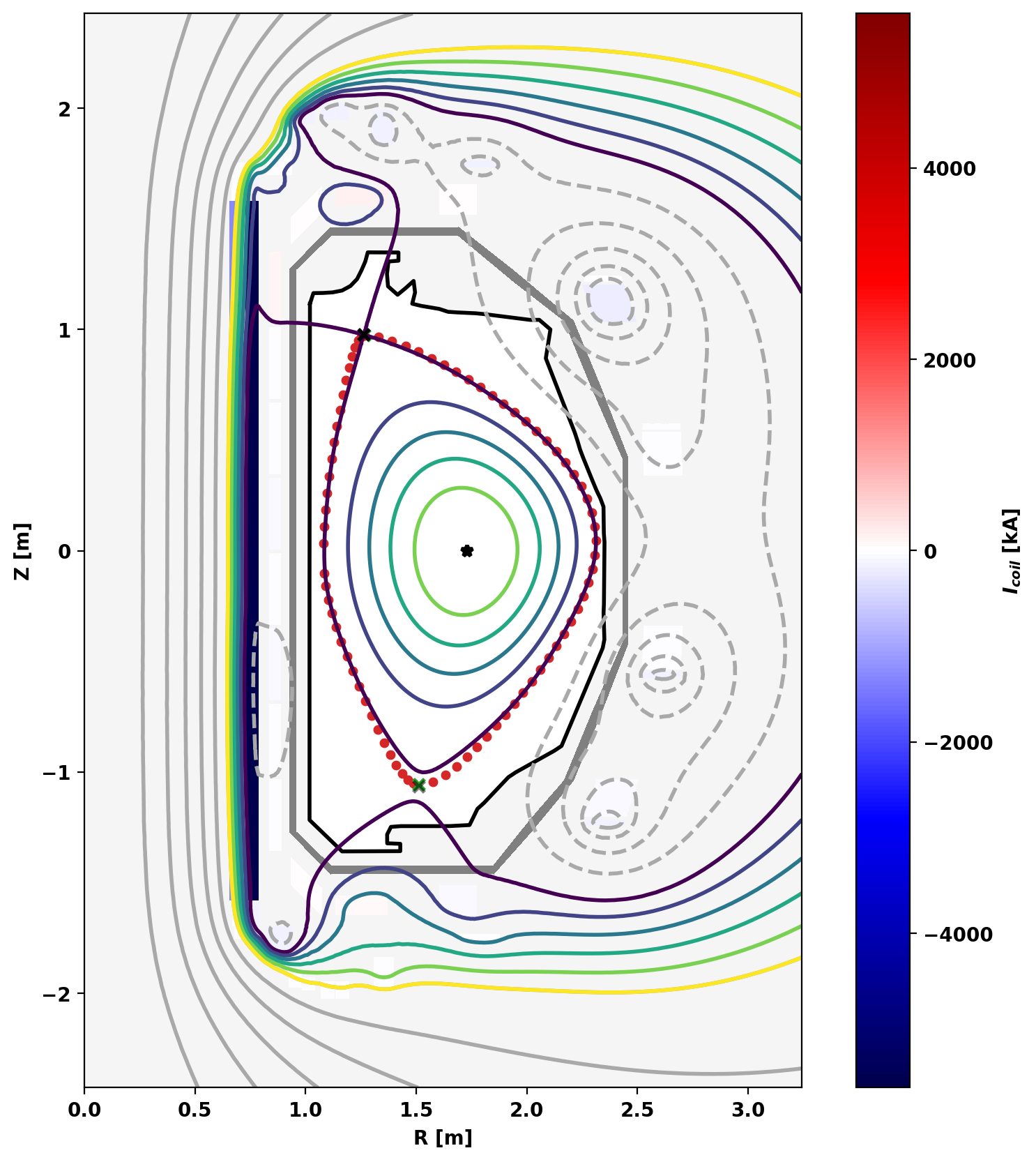
Basic parameters can be displayed using the print_info() method. For access to these quantities as variables instead the get_stats() can be used.
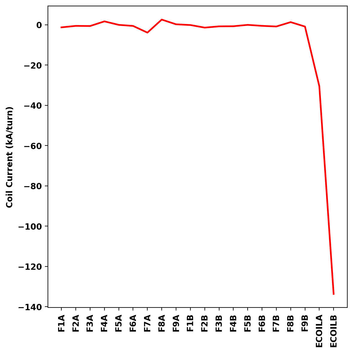
The final coil currents can also be retrieved using the get_coil_currents() method. Here, we plot the deviation of the TokaMaker currents from the desired target currents set above.
Equilibrium Statistics:
  Topology                =   Diverted
  Toroidal Current [A]    =    5.0000E+05
  Current Centroid [m]    =    1.679 -0.003
  Magnetic Axis [m]       =    1.728 -0.001
  Elongation              =    1.609 (U:  1.589, L:  1.630)
  Triangularity           =    0.487 (U:  0.709, L:  0.266)
  Plasma Volume [m^3]     =   17.009
  q_0, q_95               =    2.294  8.460
  Plasma Pressure [Pa]    =   Axis:  6.9912E+03, Peak:  6.9912E+03
  Stored Energy [J]       =    5.6473E+04
  <Beta_pol> [%]          =   34.6927
  <Beta_tor> [%]          =    0.1513
  <Beta_n>   [%]          =    0.3564
  Diamagnetic flux [Wb]   =    5.1948E-03
  Toroidal flux [Wb]      =    3.4004E+00
  l_i                     =    1.2327
We save our TokaMaker equilibrium as a gEQDSK file using the save_eqdsk() method. We modify the resolution of the equilibrium file by increasing the nr and nz parameters and decreasing the padding on the last closed flux surface (lcfs_pad).
Saving gEQDSK: g999999_tokamaker
 1.17.0