In this example we show how to use voltage-specified coils
This example utilizes the mesh built in TokaMaker Meshing Example: Building a mesh for HBT-EP.
- Note
- Running this example requires the h5py python package, which is installable using pip or other standard methods.
import os
import sys
import copy
import numpy as np
import matplotlib.pyplot as plt
plt.rcParams['figure.figsize']=(6,6)
plt.rcParams['font.weight']='bold'
plt.rcParams['axes.labelweight']='bold'
plt.rcParams['lines.linewidth']=2
plt.rcParams['lines.markeredgewidth']=2
%matplotlib inline
%config InlineBackend.figure_format = "retina"
Load TokaMaker library
To load the TokaMaker python module we need to tell python where to the module is located. This can be done either through the PYTHONPATH environment variable or using within a script using sys.path.append() as below, where we look for the environement variable OFT_ROOTPATH to provide the path to where the OpenFUSIONToolkit is installed (/Applications/OFT on macOS).
For meshing we will use the gs_Domain() class to build a 2D triangular grid suitable for Grad-Shafranov equilibria. This class uses the triangle code through a python wrapper.
tokamaker_python_path = os.getenv('OFT_ROOTPATH')
if tokamaker_python_path is not None:
sys.path.append(os.path.join(tokamaker_python_path,'python'))
from OpenFUSIONToolkit import OFT_env
Setup model
Initialize OFT environment
We now create a OFT_env instance for execution using two threads. This environment will be shared by both our TokaMaker models below.
myOFT = OFT_env(nthreads=2)
#----------------------------------------------
             ____  ____________
            / __ \/ ____/_  __/
           / / / / /_    / /
          / /_/ / __/   / /
          \____/_/     /_/

Base release:        v1.0.0-beta7
Development branch:  release_26_06
Revision id:         978c4b9f

Parallelization Info:
  Not compiled with MPI
  # of OpenMP threads =    2

Linear Algebra backend: native

#----------------------------------------------
Build two TokaMaker models
To illustrate the use of Vcoils we build two models of HBT-EP: 1) The full model of HBT-EP with passive conducting regions (VV, Shell) and 2) A reduced model with high resistivity in the VV and Shell, which can be reproduced with a simple L-R ODE.
We use the same mesh for both models, generated in TokaMaker Meshing Example: Building a mesh for HBT-EP and loaded using load_gs_mesh(). Before calling setup_regions() on the simplified model we set the resistivity to large values in the VV and Shell.
mesh_pts,mesh_lc,mesh_reg,coil_dict,cond_dict = load_gs_mesh('HBT_mesh.h5')
mygs_full = TokaMaker(myOFT)
mygs_full.setup_mesh(mesh_pts, mesh_lc, mesh_reg)
mygs_full.setup_regions(cond_dict=cond_dict,coil_dict=coil_dict)
mygs_full.setup(order=3, F0=0.2518*1.23)
mygs_nocond = TokaMaker(myOFT)
cond_dict_nocond = copy.deepcopy(cond_dict)
cond_dict_nocond['VV']['eta'] = 1.E4
cond_dict_nocond['SHELL']['eta'] = 1.E4
mygs_nocond.setup_mesh(mesh_pts, mesh_lc, mesh_reg)
mygs_nocond.setup_regions(cond_dict=cond_dict_nocond,coil_dict=coil_dict)
mygs_nocond.setup(order=3, F0=0.2518*1.23)
**** Loading OFT surface mesh

**** Generating surface grid level  1
  Generating boundary domain linkage
  Mesh statistics:
    Area         =  3.278E+00
    # of points  =    3736
    # of edges   =   11087
    # of cells   =    7352
    # of boundary points =     118
    # of boundary edges  =     118
    # of boundary cells  =     118
  Resolution statistics:
    hmin =  1.959E-04
    hrms =  3.418E-02
    hmax =  9.532E-02
  Surface grounded at vertex     804


**** Creating Lagrange FE space
  Order  =    3
  Minlev =   -1

 Computing flux BC matrix
 Inverting real matrix
   Time =    2.3400000000000001E-003

**** Loading OFT surface mesh

**** Generating surface grid level  1
  Generating boundary domain linkage
  Mesh statistics:
    Area         =  3.278E+00
    # of points  =    3736
    # of edges   =   11087
    # of cells   =    7352
    # of boundary points =     118
    # of boundary edges  =     118
    # of boundary cells  =     118
  Resolution statistics:
    hmin =  1.959E-04
    hrms =  3.418E-02
    hmax =  9.532E-02
  Surface grounded at vertex     804


**** Creating Lagrange FE space
  Order  =    3
  Minlev =   -1

 Computing flux BC matrix
 Inverting real matrix
   Time =    2.2209999999999999E-003
Run simplified model
mygs = mygs_nocond
mygs.settings.pm=False
mygs.update_settings()
mygs.set_coil_currents({'OH': 1.E3})
eq_vac = mygs.vac_solve()
psi_vac = eq_vac.get_psi(False)
rcoils = {'OH': 10.E-3, 'VF': 10.E-3}
mygs.set_vcoils(rcoils)
coils_volt = {'OH': 0.0}
dt=1.E-3
new_coil_currents, _ = mygs.get_coil_currents()
psi_new = psi_vac.copy()
coil_hist = [mygs.coil_dict2vec(new_coil_currents),]
for i in range(160):
mygs.set_psi_dt(psi_new,dt,new_coil_currents,coils_volt)
eq_new = mygs.vac_solve()
psi_new = eq_new.get_psi(False)
new_coil_currents, _ = eq_new.get_coil_currents()
coil_hist.append(mygs.coil_dict2vec(new_coil_currents))
coil_hist = np.array(coil_hist)
mygs.settings.pm=True
mygs.update_settings()
WARNING: TokaMaker's Vcoil functionality is experimental, use with caution and report bugs
Repeat using NL solver
Verify NL solver works correctly, but system itself is still linear
mygs.settings.pm=False
mygs.update_settings()
mygs.set_coil_currents({'OH': 1.E3})
mygs.set_psi(psi_vac)
coil_hist_nl = [mygs.coil_dict2vec(mygs.get_coil_currents()[0])]
mygs.setup_td(dt,1.E-13,1.E-11,pre_plasma=False)
sim_time = 0.0
for i in range(160):
sim_time, _, nl_its, lin_its, nretry = mygs.step_td(sim_time,dt)
coil_hist_nl.append(mygs.coil_dict2vec(mygs.get_coil_currents()[0]))
coil_hist_nl = np.array(coil_hist_nl)
mygs.settings.pm=True
mygs.update_settings()
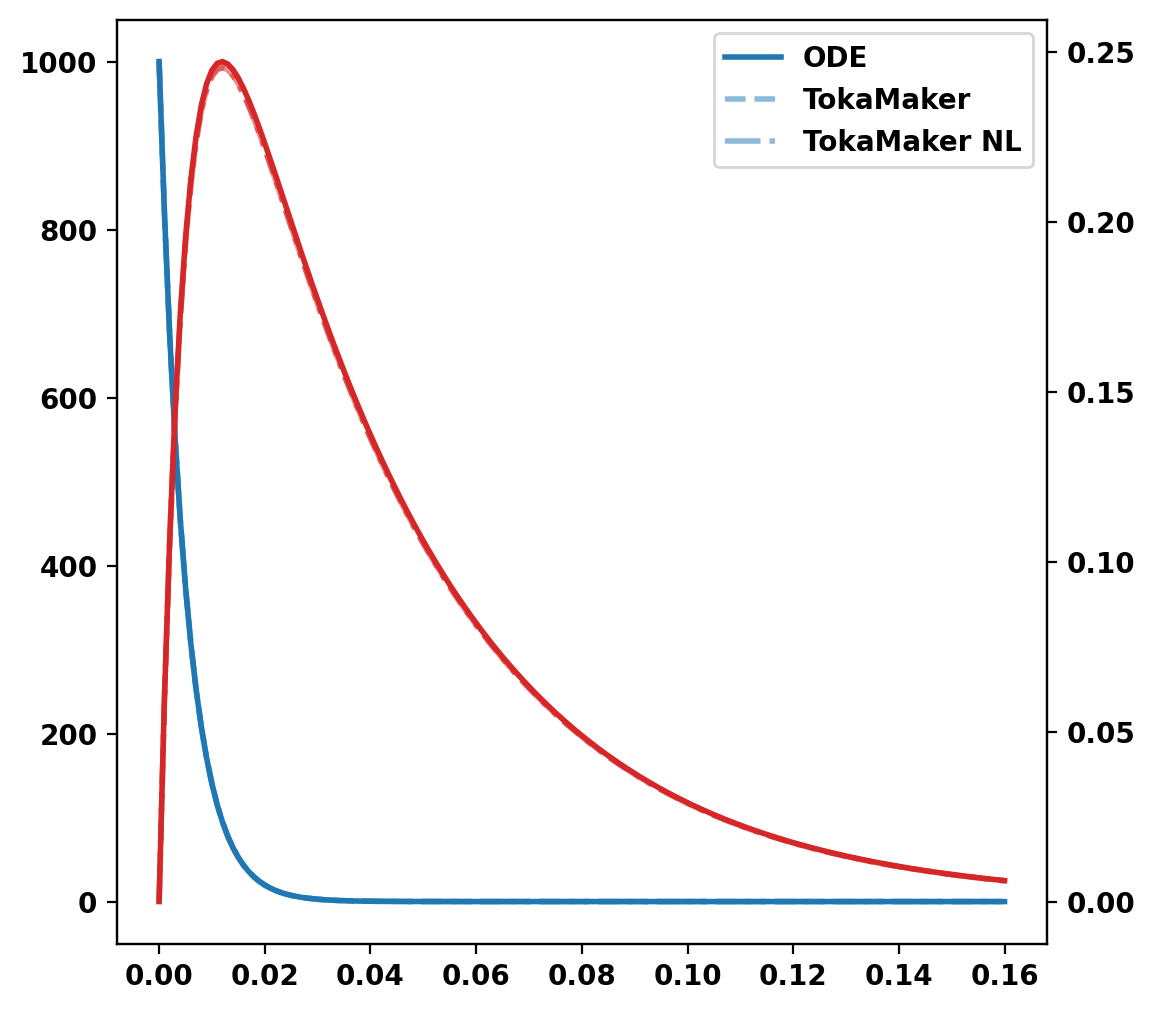
Compute L-R ODE comparison
This system should behave as a simple 2x2 ODE for the OH and VF coils.
Lmat = mygs.get_coil_Lmat()[:-1,:-1]
Lmat[:,-1]=0.0; Lmat[-1,:]=0.0; Lmat[-1,-1] = 1.0
Rmat=np.diag(mygs.coil_dict2vec(rcoils))
new_coil_simple = coil_hist[0]
analytic_op = np.linalg.inv(Lmat+dt*Rmat)
coil_hist_simple = [new_coil_simple,]
for i in range(160):
volt_vec=mygs.coil_dict2vec(coils_volt)
new_coil_simple = np.dot(analytic_op,dt*volt_vec+np.dot(Lmat,new_coil_simple))
coil_hist_simple.append(new_coil_simple)
coil_hist_simple = np.array(coil_hist_simple)
Starting LU solver: umfpack F
Compare TokaMaker and ODE results
fig, ax = plt.subplots(1,1)
time = np.cumsum(dt*np.ones((len(coil_hist_simple),)))-dt
ax.plot(time,coil_hist_simple[:,0],color='tab:blue',label='ODE')
ax.plot(time,coil_hist[:,0],'--',color='tab:blue',alpha=0.5,label='TokaMaker')
ax.plot(time,coil_hist_nl[:,0],'-.',color='tab:blue',alpha=0.5,label='TokaMaker NL')
ax2=ax.twinx()
ax2.plot(time,coil_hist_simple[:,1],color='tab:red')
ax2.plot(time,coil_hist[:,1],'--',color='tab:red',alpha=0.5)
ax2.plot(time,coil_hist_nl[:,1],'-.',color='tab:red',alpha=0.5)
_ = ax.legend()
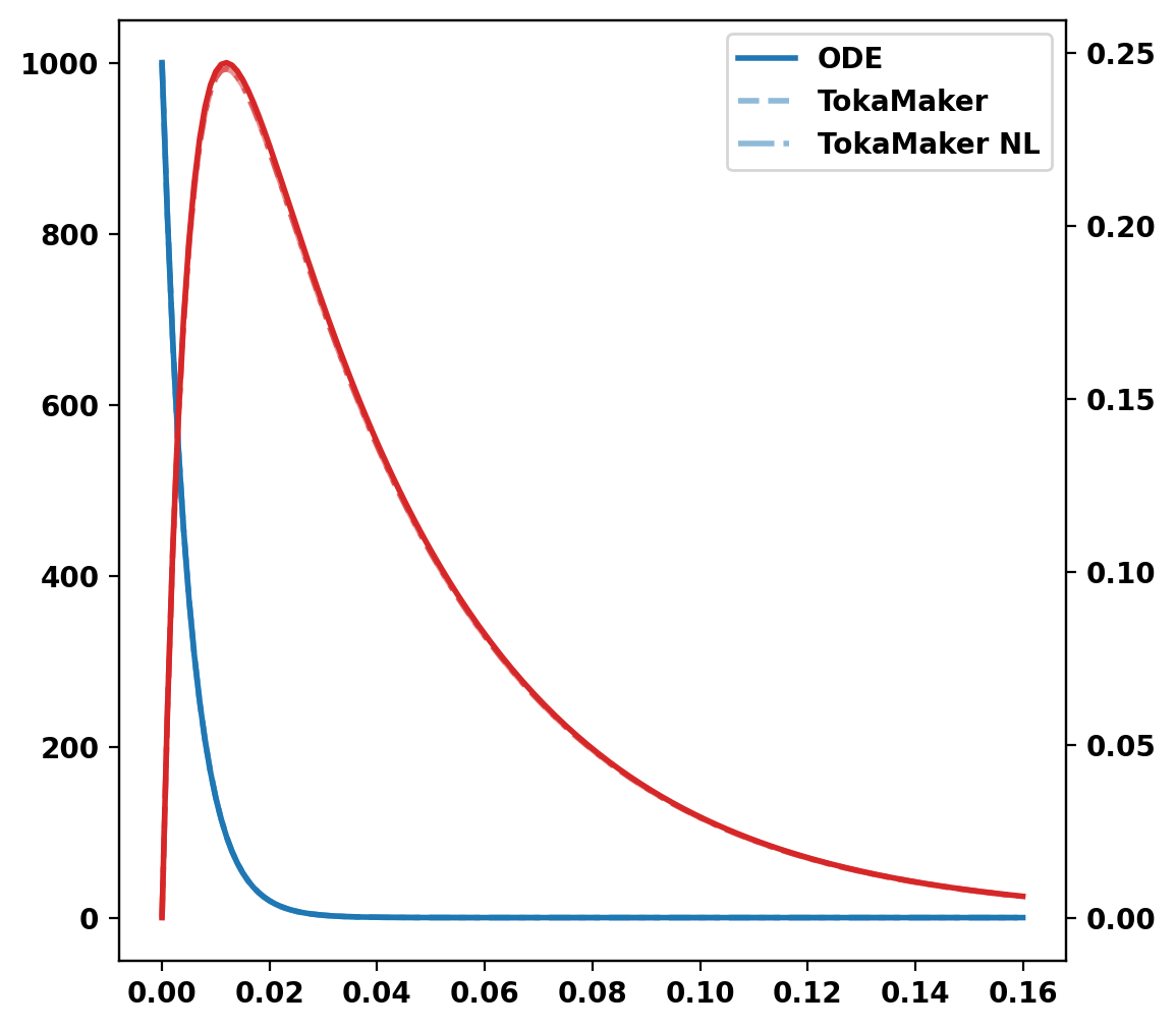
Repeat with one Icoil and one Vcoil
mygs.settings.pm=False
mygs.update_settings()
mygs.set_psi_dt(psi_new,2.0*dt,new_coil_currents,coils_volt)
psi_vac = mygs.vac_solve()
mygs.set_psi_dt(psi_new,-dt,new_coil_currents,coils_volt)
mygs.set_coil_currents({'OH': 1.E3})
eq_vac = mygs.vac_solve()
psi_vac = eq_vac.get_psi(False)
rcoils = {'VF': 10.E-3}
mygs.set_vcoils(rcoils)
coils_volt = {}
dt=1.E-3
old_coil_currents, _ = mygs.get_coil_currents()
psi_new = psi_vac.copy()
coil_hist = [mygs.coil_dict2vec(old_coil_currents),]
for i in range(159):
mygs.set_psi_dt(psi_new,dt,old_coil_currents,coils_volt)
new_coil_currents = copy.deepcopy(old_coil_currents); new_coil_currents['OH'] = coil_hist_simple[i+1,0]
mygs.set_coil_currents(new_coil_currents)
eq_new = mygs.vac_solve()
psi_new = eq_new.get_psi(False)
old_coil_currents, _ = mygs.get_coil_currents()
coil_hist.append(mygs.coil_dict2vec(old_coil_currents))
coil_hist = np.array(coil_hist)
mygs.settings.pm=True
mygs.update_settings()
Repeat using NL solver
Verify NL solver works correctly, but system itself is still linear
mygs.set_coil_currents({'OH': 1.E3})
mygs.set_psi(psi_vac)
old_coil_currents, _ = mygs.get_coil_currents()
coil_hist_nl = [mygs.coil_dict2vec(old_coil_currents)]
mygs.settings.pm=False
mygs.update_settings()
mygs.setup_td(dt,1.E-13,1.E-11,pre_plasma=False)
sim_time = 0.0
for i in range(159):
new_coil_currents = copy.deepcopy(old_coil_currents); new_coil_currents['OH'] = coil_hist_simple[i+1,0]
sim_time, _, nl_its, lin_its, nretry = mygs.step_td(sim_time,dt,coil_currents=new_coil_currents)
old_coil_currents, _ = mygs.get_coil_currents()
coil_hist_nl.append(mygs.coil_dict2vec(old_coil_currents))
coil_hist_nl = np.array(coil_hist_nl)
mygs.settings.pm=True
mygs.update_settings()
Compare to ODE results
fig, ax = plt.subplots(1,1)
time = np.cumsum(dt*np.ones((len(coil_hist_simple),)))-dt
ax.plot(time,coil_hist_simple[:,0],color='tab:blue',label='ODE')
ax.plot(time[:-1],coil_hist[:,0],'--',color='tab:blue',alpha=0.5,label='TokaMaker')
ax.plot(time[:-1],coil_hist_nl[:,0],'-.',color='tab:blue',alpha=0.5,label='TokaMaker NL')
ax2=ax.twinx()
ax2.plot(time,coil_hist_simple[:,1],color='tab:red')
ax2.plot(time[:-1],coil_hist[:,1],'--',color='tab:red',alpha=0.5)
ax2.plot(time[:-1],coil_hist_nl[:,1],'-.',color='tab:red',alpha=0.5)
_ = ax.legend()
Run full model
mygs = mygs_full
mygs.settings.pm=False
mygs.update_settings()
mygs.set_coil_currents({'OH': 1.E3})
eq_vac = mygs.vac_solve()
psi_vac = eq_vac.get_psi(False)
rcoils = {'OH': 10.E-3, 'VF': 10.E-3}
mygs.set_vcoils(rcoils)
coils_volt = {'OH': 0.0}
dt=1.E-3
new_coil_currents, _ = mygs.get_coil_currents()
psi_new = psi_vac.copy()
coil_hist = [mygs.coil_dict2vec(new_coil_currents),]
for i in range(160):
mygs.set_psi_dt(psi_new,dt,new_coil_currents,coils_volt)
eq_new = mygs.vac_solve()
psi_new = eq_new.get_psi(False)
new_coil_currents, _ = mygs.get_coil_currents()
coil_hist.append(mygs.coil_dict2vec(new_coil_currents))
coil_hist = np.array(coil_hist)
mygs.settings.pm=True
mygs.update_settings()
WARNING: TokaMaker's Vcoil functionality is experimental, use with caution and report bugs
Repeat using NL solver
Verify NL solver works correctly, but system itself is still linear
mygs.settings.pm=False
mygs.update_settings()
mygs.set_coil_currents({'OH': 1.E3})
mygs.set_psi(psi_vac)
coil_hist_nl = [mygs.coil_dict2vec(mygs.get_coil_currents()[0])]
mygs.setup_td(dt,1.E-13,1.E-11,pre_plasma=False)
sim_time = 0.0
for i in range(160):
sim_time, _, nl_its, lin_its, nretry = mygs.step_td(sim_time,dt)
coil_hist_nl.append(mygs.coil_dict2vec(mygs.get_coil_currents()[0]))
coil_hist_nl = np.array(coil_hist_nl)
mygs.settings.pm=True
mygs.update_settings()
Compute L-R ODE comparison
new_coil_simple = coil_hist[0]
coil_hist_simple = [new_coil_simple,]
for i in range(160):
volt_vec=mygs.coil_dict2vec(coils_volt)
new_coil_simple = np.dot(analytic_op,dt*volt_vec+np.dot(Lmat,new_coil_simple))
coil_hist_simple.append(new_coil_simple)
coil_hist_simple = np.array(coil_hist_simple)
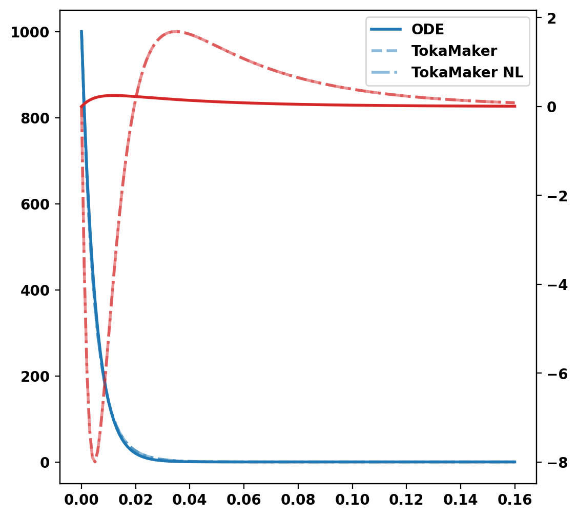
Compare TokaMaker and ODE results
In this case the TokaMaker and ODE results should only agree late in time, since the ODE does not include the VV or Shell.
fig, ax = plt.subplots(1,1)
time = np.cumsum(dt*np.ones((len(coil_hist),)))-dt
ax.plot(time,coil_hist_simple[:,0],color='tab:blue',label='ODE')
ax.plot(time,coil_hist[:,0],'--',color='tab:blue',alpha=0.5,label='TokaMaker')
ax.plot(time,coil_hist_nl[:,0],'-.',color='tab:blue',alpha=0.5,label='TokaMaker NL')
ax2=ax.twinx()
ax2.plot(time,coil_hist_simple[:,1],color='tab:red')
ax2.plot(time,coil_hist[:,1],'--',color='tab:red',alpha=0.5)
ax2.plot(time,coil_hist_nl[:,1],'-.',color='tab:red',alpha=0.5)
_ = ax.legend()
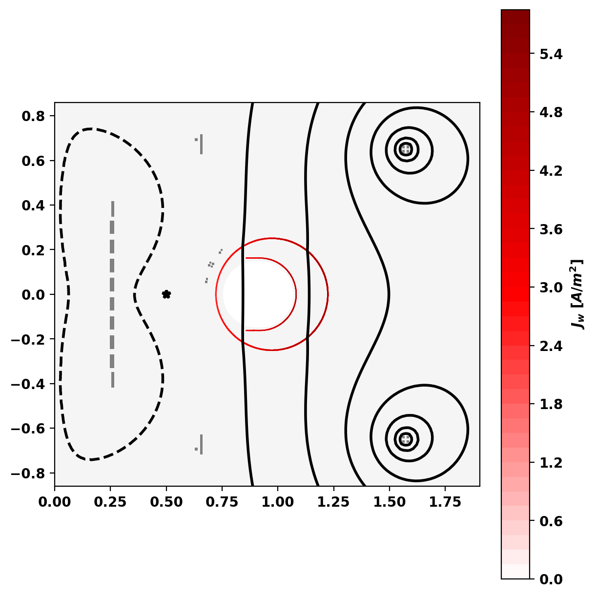
Plot eddy currents
fig, ax = plt.subplots(1,1,constrained_layout=True)
mygs.plot_machine(fig,ax,coil_colormap=None,limiter_color=None)
mygs.plot_psi(fig,ax,psi=psi_new,normalized=False,plasma_nlevels=10,plasma_color='k',vacuum_levels=None,xpoint_color=None)
_ = mygs.plot_eddy(fig,ax,psi=psi_new,colormap='seismic',symmap=True)
Starting CG solver
     0  0.000000E+00  0.000000E+00  1.691097E-07
     1 -7.873203E-10  1.353692E-02  8.254653E-08  6.097883E-06
     2 -8.360726E-10  1.333031E-02  4.042682E-08  3.032699E-06
     3 -8.513913E-10  1.337349E-02  1.995725E-08  1.492299E-06
     4 -8.548581E-10  1.363831E-02  1.012042E-08  7.420587E-07
     5 -8.554565E-10  1.379286E-02  4.460942E-09  3.234240E-07
     6 -8.555727E-10  1.380921E-02  2.220260E-09  1.607811E-07
     7 -8.555953E-10  1.380685E-02  1.144602E-09  8.290101E-08
     8 -8.556020E-10  1.380955E-02  4.359230E-10  3.156678E-08
     9 -8.556029E-10  1.381139E-02  1.686939E-10  1.221411E-08
    10 -8.556030E-10  1.381141E-02  9.536271E-11  6.904631E-09
    20 -8.556031E-10  1.381056E-02  2.811696E-14  2.035903E-12
Repeat with one Icoil and one Vcoil
mygs.settings.pm=False
mygs.update_settings()
mygs.set_psi_dt(psi_new,2.0*dt,new_coil_currents,coils_volt)
psi_vac = mygs.vac_solve()
mygs.set_psi_dt(psi_new,-dt,new_coil_currents,coils_volt)
mygs.set_coil_currents({'OH': 1.E3})
eq_vac = mygs.vac_solve()
psi_vac = eq_vac.get_psi(False)
rcoils = {'VF': 10.E-3}
mygs.set_vcoils(rcoils)
coils_volt = {}
dt=1.E-3
old_coil_currents, _ = mygs.get_coil_currents()
psi_new = psi_vac.copy()
coil_hist_new = [mygs.coil_dict2vec(old_coil_currents),]
for i in range(159):
mygs.set_psi_dt(psi_new,dt,old_coil_currents,coils_volt)
new_coil_currents = copy.deepcopy(old_coil_currents); new_coil_currents['OH'] = coil_hist[i+1,0]
mygs.set_coil_currents(new_coil_currents)
eq_vac = mygs.vac_solve()
psi_new = eq_vac.get_psi(False)
old_coil_currents, _ = mygs.get_coil_currents()
coil_hist_new.append(mygs.coil_dict2vec(old_coil_currents))
coil_hist_new = np.array(coil_hist_new)
mygs.settings.pm=True
mygs.update_settings()
Repeat using NL solver
Verify NL solver works correctly, but system itself is still linear
mygs.set_coil_currents({'OH': 1.E3})
mygs.set_psi(psi_vac)
old_coil_currents, _ = mygs.get_coil_currents()
coil_hist_nl = [mygs.coil_dict2vec(old_coil_currents)]
mygs.settings.pm=False
mygs.update_settings()
mygs.setup_td(dt,1.E-13,1.E-11,pre_plasma=False)
sim_time = 0.0
for i in range(159):
new_coil_currents = copy.deepcopy(old_coil_currents); new_coil_currents['OH'] = coil_hist[i+1,0]
sim_time, _, nl_its, lin_its, nretry = mygs.step_td(sim_time,dt,coil_currents=new_coil_currents)
old_coil_currents, _ = mygs.get_coil_currents()
coil_hist_nl.append(mygs.coil_dict2vec(old_coil_currents))
coil_hist_nl = np.array(coil_hist_nl)
mygs.settings.pm=True
mygs.update_settings()
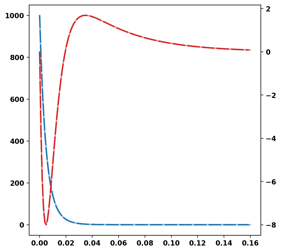
Compare Vcoil and Icoil results
fig, ax = plt.subplots(1,1)
time = np.cumsum(dt*np.ones((len(coil_hist),)))-dt
ax.plot(time,coil_hist[:,0],color='tab:blue',alpha=0.5)
ax.plot(time[:-1],coil_hist_new[:,0],'--',color='tab:blue')
ax.plot(time[:-1],coil_hist_nl[:,0],'-.',color='tab:blue')
ax2=ax.twinx()
ax2.plot(time,coil_hist[:,1],color='tab:red',alpha=0.5)
ax2.plot(time[:-1],coil_hist_new[:,1],'--',color='tab:red')
_ = ax2.plot(time[:-1],coil_hist_nl[:,1],'-.',color='tab:red')

 1.17.0