 |
The Open FUSION Toolkit 26.9
An open-source framework for fusion and plasma science and engineering
|
Loading...
Searching...
No Matches
|
The Open FUSION Toolkit 26.9
An open-source framework for fusion and plasma science and engineering
|
Ohmic start-up needs three things to line up at the same place and time:
(a) A poloidal-field null. The central solenoid (CS) ramps down to drive a toroidal loop voltage \(V_{loop} = 2\pi R\,E_\phi\). The CS and PF coils also make a stray poloidal field; where it cancels, \(|B_{pol}|\to 0\) (a field null) and field lines become nearly purely toroidal. A freshly-ionized electron then stays in the chamber for a long connection length \(\)L_c \approx 0.25\,a\,\frac{B_\phi}{B_T}, \(\) where \(a\) is the size of the low-field region, \(B_\phi\) the toroidal field, and \(B_T\) the (average) stray poloidal field over the null region. A good null keeps \(B_T\) small here (~1 mT).
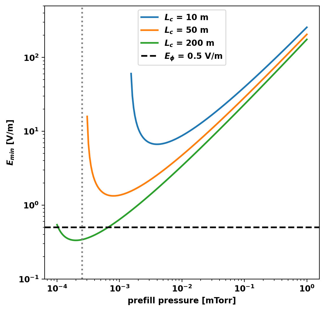
(b) Townsend avalanche. Seed electrons accelerated by \(E_\phi\) ionize the prefill gas, and then the the electron density grows via Townsend avalance. Requiring at least one e-folding, \(\alpha L_c \ge 1\), gives a Paschen-type minimum field \(E_{min}(p)=Bp/\ln(A\,p\,L_c)\), which is smallest at a particular prefill pressure (the Paschen minimum).
(c) Loop voltage and the engineering criterion. The CS flux swing must supply \(V_{loop}=2\pi R\,E_\phi\). The tokamak start-up community compresses (a)–(b) into two experimentally-calibrated rules (Leuer et al. 2010): \(E_\phi \ge 0.3\) V/m (ohmic, 0.15 with ECRF) and \(E_\phi B_\phi / B_T \ge 10^{3}\) V/m.
#----------------------------------------------
Open FUSION Toolkit Initialized
Development branch:    arc_v3a
Revision id:           04589ca
Parallelization Info:
  Not compiled with MPI
  # of OpenMP threads =    2
Integer Precisions    =    4   8
Float Precisions      =    4   8  16
Complex Precisions    =    4   8
LA backend            = native
#----------------------------------------------
**** Loading OFT surface mesh

**** Generating surface grid level  1
  Generating boundary domain linkage
  Mesh statistics:
    Area         =  1.301E+00
    # of points  =    5796
    # of edges   =   17283
    # of cells   =   11488
    # of boundary points =     102
    # of boundary edges  =     102
    # of boundary cells  =     102
  Resolution statistics:
    hmin =  3.994E-03
    hrms =  1.721E-02
    hmax =  7.410E-02
  Surface grounded at vertex     761


**** Creating Lagrange FE space
  Order  =    2
  Minlev =   -1

 Computing flux BC matrix
 Inverting real matrix
   Time =    4.9899999999999999E-004
For breakdown studies, the coil limits set the maximum availble flux (described below).
Starting non-linear GS solver
     1  4.8509E-02  3.6569E-02  1.7441E-05  2.0845E-01 -4.8889E-06 -0.0000E+00
     2  5.4935E-02  3.8654E-02  4.0467E-06  2.0778E-01 -2.3793E-06 -0.0000E+00
     3  5.7506E-02  3.9451E-02  1.2647E-06  2.0756E-01 -1.7281E-06 -0.0000E+00
     4  5.8597E-02  3.9771E-02  4.9556E-07  2.0749E-01 -1.5233E-06 -0.0000E+00
 Timing:   3.8020999636501074E-002
   Source:     1.6634999774396420E-002
   Solve:      7.0819999091327190E-003
   Boundary:   1.3500000350177288E-003
   Other:      1.2953999917954206E-002
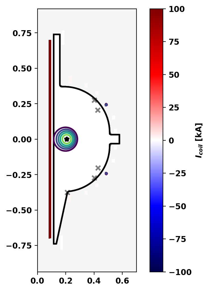
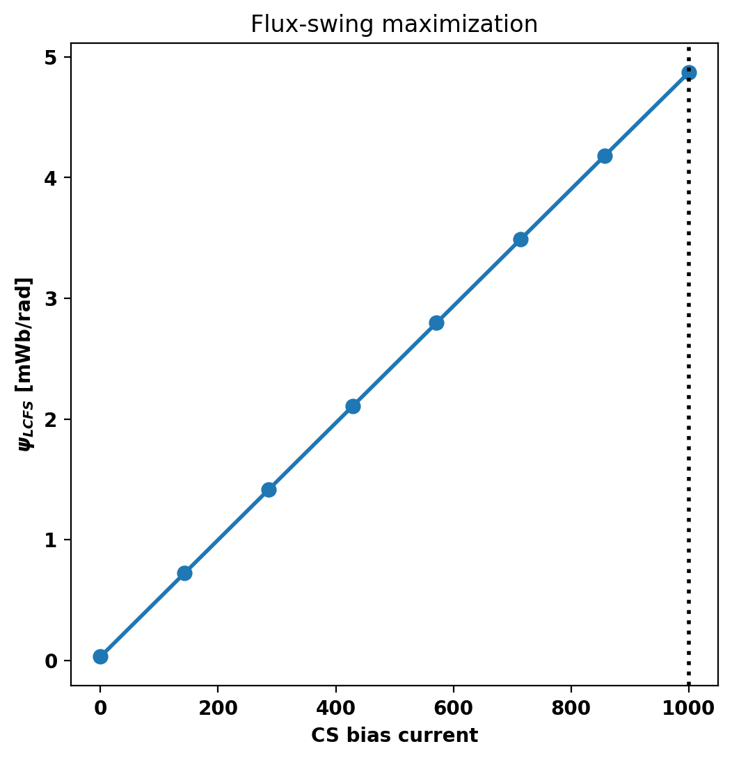
\(\psi_{LCFS}\) is the poloidal flux on the plasma boundary. The central solenoid (CS) acts as the primary of a transformer: its changing flux drives the loop voltage \(V_{loop} = -d\psi/dt\) that ionizes the gas and sustains \(I_p\). The total volt-second budget for the discharge is the availailible flux swing \(\Delta\psi\) between the fully-biased CS state at breakdown and the most negative \(\psi\) reachable at the end of the ramp.
The more boundary flux we can establish at breakdown, more flux swing we have availible for the pulse. Effectively this means that we want to bias the CS stack as hard as the coil-current limits allow. Here we scans the CS bias current, re-solve the equilibrium at each value, and keep the bias that gives the largest \(\psi_{LCFS}\) (then re-solves there so the rest of the notebook uses that state).
Starting non-linear GS solver
     1  4.8418E-02  3.6506E-02  1.5653E-05  2.0844E-01 -9.9305E-06 -0.0000E+00


/var/folders/77/9hnl3h2d5jq7v8mv35f7n_z40000gn/T/ipykernel_42417/988288092.py:24: DeprecationWarning: `set_isoflux()` is deprecated, use `set_isoflux_constraints()` instead. This function will be removed in a future version.
  mygs.set_isoflux(isoflux_pts)
/var/folders/77/9hnl3h2d5jq7v8mv35f7n_z40000gn/T/ipykernel_42417/988288092.py:25: DeprecationWarning: `set_saddles()` is deprecated, use `set_saddle_constraints()` instead. This function will be removed in a future version.
  mygs.set_saddles(None)


     2  5.4828E-02  3.8589E-02  4.2606E-06  2.0777E-01 -7.5875E-06 -0.0000E+00
     3  5.7395E-02  3.9384E-02  1.3790E-06  2.0755E-01 -7.0146E-06 -0.0000E+00
     4  5.8483E-02  3.9704E-02  5.1992E-07  2.0747E-01 -6.8365E-06 -0.0000E+00
 Timing:   3.8477999623864889E-002
   Source:     1.6958001069724560E-002
   Solve:      8.0989999696612358E-003
   Boundary:   9.1899931430816650E-004
   Other:      1.2501999270170927E-002
Starting non-linear GS solver
     1  4.8431E-02  3.6515E-02  1.5904E-05  2.0844E-01 -9.2441E-06 -0.0000E+00
     2  5.4843E-02  3.8598E-02  4.2324E-06  2.0777E-01 -6.8762E-06 -0.0000E+00
     3  5.7410E-02  3.9393E-02  1.3613E-06  2.0755E-01 -6.2918E-06 -0.0000E+00
     4  5.8499E-02  3.9714E-02  5.1522E-07  2.0747E-01 -6.1098E-06 -0.0000E+00
 Timing:   3.6767000332474709E-002
   Source:     1.6302999574691057E-002
   Solve:      7.0689995773136616E-003
   Boundary:   8.7000103667378426E-004
   Other:      1.2525000143796206E-002
Starting non-linear GS solver
     1  4.8444E-02  3.6524E-02  1.6158E-05  2.0844E-01 -8.5578E-06 -0.0000E+00
     2  5.4858E-02  3.8607E-02  4.2044E-06  2.0777E-01 -6.1650E-06 -0.0000E+00
     3  5.7426E-02  3.9402E-02  1.3442E-06  2.0755E-01 -5.5693E-06 -0.0000E+00
     4  5.8515E-02  3.9723E-02  5.1091E-07  2.0748E-01 -5.3832E-06 -0.0000E+00
 Timing:   3.6133000161498785E-002
   Source:     1.5830000396817923E-002
   Solve:      6.7030000500380993E-003
   Boundary:   9.2900078743696213E-004
   Other:      1.2670998927205801E-002
Starting non-linear GS solver
     1  4.8456E-02  3.6532E-02  1.6414E-05  2.0844E-01 -7.8718E-06 -0.0000E+00
     2  5.4873E-02  3.8616E-02  4.1767E-06  2.0778E-01 -5.4542E-06 -0.0000E+00
     3  5.7442E-02  3.9412E-02  1.3280E-06  2.0756E-01 -4.8471E-06 -0.0000E+00
     4  5.8531E-02  3.9732E-02  5.0718E-07  2.0748E-01 -4.6569E-06 -0.0000E+00
 Timing:   3.6399000324308872E-002
   Source:     1.5922999475151300E-002
   Solve:      6.7830001935362816E-003
   Boundary:   9.6800085157155991E-004
   Other:      1.2724999804049730E-002
Starting non-linear GS solver
     1  4.8469E-02  3.6541E-02  1.6671E-05  2.0844E-01 -7.1860E-06 -0.0000E+00
     2  5.4888E-02  3.8625E-02  4.1494E-06  2.0778E-01 -4.7437E-06 -0.0000E+00
     3  5.7457E-02  3.9421E-02  1.3126E-06  2.0756E-01 -4.1253E-06 -0.0000E+00
     4  5.8547E-02  3.9742E-02  5.0389E-07  2.0748E-01 -3.9310E-06 -0.0000E+00
 Timing:   3.5846000071614981E-002
   Source:     1.5581999905407429E-002
   Solve:      6.7280000075697899E-003
   Boundary:   9.1900071129202843E-004
   Other:      1.2616999447345734E-002
Starting non-linear GS solver
     1  4.8482E-02  3.6550E-02  1.6930E-05  2.0844E-01 -6.5002E-06 -0.0000E+00
     2  5.4903E-02  3.8635E-02  4.1221E-06  2.0778E-01 -4.0332E-06 -0.0000E+00
     3  5.7473E-02  3.9430E-02  1.2980E-06  2.0756E-01 -3.4031E-06 -0.0000E+00
     4  5.8562E-02  3.9751E-02  5.0109E-07  2.0748E-01 -3.2050E-06 -0.0000E+00
 Timing:   3.6028000060468912E-002
   Source:     1.5740000177174807E-002
   Solve:      6.7010000348091125E-003
   Boundary:   1.1560004204511642E-003
   Other:      1.2430999428033829E-002
Starting non-linear GS solver
     1  4.8495E-02  3.6559E-02  1.7191E-05  2.0845E-01 -5.8144E-06 -0.0000E+00
     2  5.4918E-02  3.8644E-02  4.0952E-06  2.0778E-01 -3.3224E-06 -0.0000E+00
     3  5.7488E-02  3.9440E-02  1.2843E-06  2.0756E-01 -2.6806E-06 -0.0000E+00
     4  5.8578E-02  3.9761E-02  4.9872E-07  2.0748E-01 -2.4789E-06 -0.0000E+00
 Timing:   3.5980999935418367E-002
   Source:     1.5635999385267496E-002
   Solve:      6.5390006639063358E-003
   Boundary:   1.0919999331235886E-003
   Other:      1.2713999953120947E-002
Starting non-linear GS solver
     1  4.8509E-02  3.6569E-02  1.7441E-05  2.0845E-01 -4.8889E-06 -0.0000E+00
     2  5.4935E-02  3.8654E-02  4.0467E-06  2.0778E-01 -2.3793E-06 -0.0000E+00
     3  5.7506E-02  3.9451E-02  1.2647E-06  2.0756E-01 -1.7281E-06 -0.0000E+00
     4  5.8597E-02  3.9771E-02  4.9556E-07  2.0749E-01 -1.5233E-06 -0.0000E+00
 Timing:   3.6410999950021505E-002
   Source:     1.5786000527441502E-002
   Solve:      6.6389995627105236E-003
   Boundary:   1.2759994715452194E-003
   Other:      1.2710000388324261E-002
psi_LCFS:  zero-bias =  2.977E-02   maximized =  4.870E+00 [mWb/rad]
best CS bias current =  1.000E+03
Starting non-linear GS solver
     1  4.8509E-02  3.6569E-02  1.7441E-05  2.0845E-01 -4.8889E-06 -0.0000E+00
     2  5.4935E-02  3.8654E-02  4.0467E-06  2.0778E-01 -2.3793E-06 -0.0000E+00
     3  5.7506E-02  3.9451E-02  1.2647E-06  2.0756E-01 -1.7281E-06 -0.0000E+00
     4  5.8597E-02  3.9771E-02  4.9556E-07  2.0749E-01 -1.5233E-06 -0.0000E+00
 Timing:   3.6464999895542860E-002
   Source:     1.5893999952822924E-002
   Solve:      6.5440000034868717E-003
   Boundary:   1.2300000526010990E-003
   Other:      1.2796999886631966E-002
Starting non-linear GS solver
     1  5.8597E-02  3.9771E-02  3.5791E-05  2.0552E-01  1.6438E-05 -0.0000E+00
     2  5.8597E-02  3.9771E-02  7.1582E-06  1.8841E-01  3.1520E-05 -0.0000E+00
     3  5.8597E-02  3.9771E-02  1.4316E-06  5.0000E-01  0.0000E+00 -0.0000E+00
     4  5.8597E-02  3.9771E-02  2.8633E-07  5.0000E-01  0.0000E+00 -0.0000E+00
 Timing:   1.9315999932587147E-002
   Source:     0.0000000000000000
   Solve:      6.7680003121495247E-003
   Boundary:   0.0000000000000000
   Other:      1.2547999620437622E-002


/var/folders/77/9hnl3h2d5jq7v8mv35f7n_z40000gn/T/ipykernel_42417/498142008.py:2: DeprecationWarning: `set_isoflux()` is deprecated, use `set_isoflux_constraints()` instead. This function will be removed in a future version.
  mygs.set_isoflux(None)
/var/folders/77/9hnl3h2d5jq7v8mv35f7n_z40000gn/T/ipykernel_42417/498142008.py:10: DeprecationWarning: `set_saddles()` is deprecated, use `set_saddle_constraints()` instead. This function will be removed in a future version.
  mygs.set_saddles(zero_field_pts)
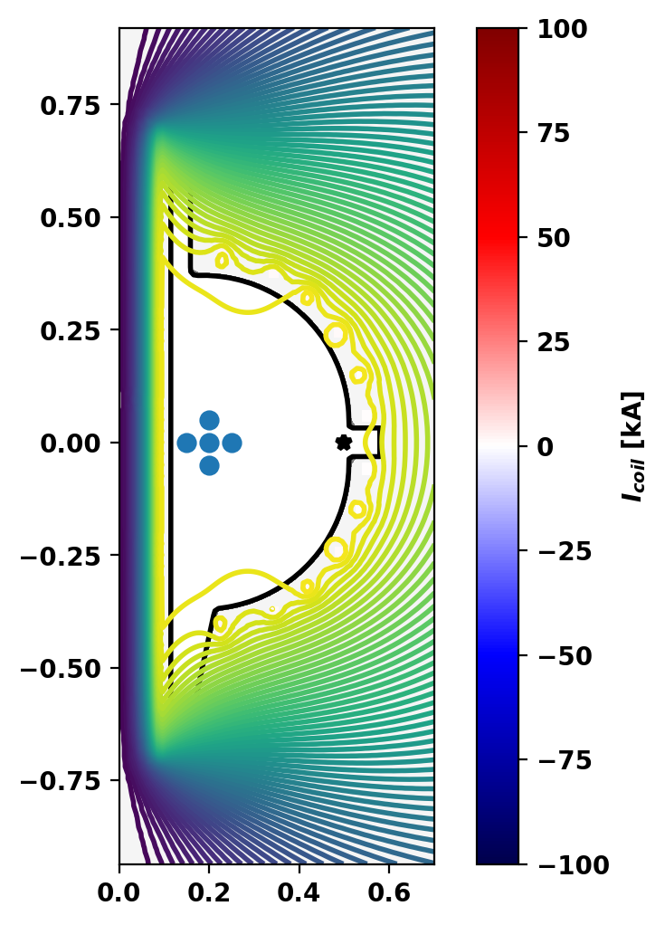
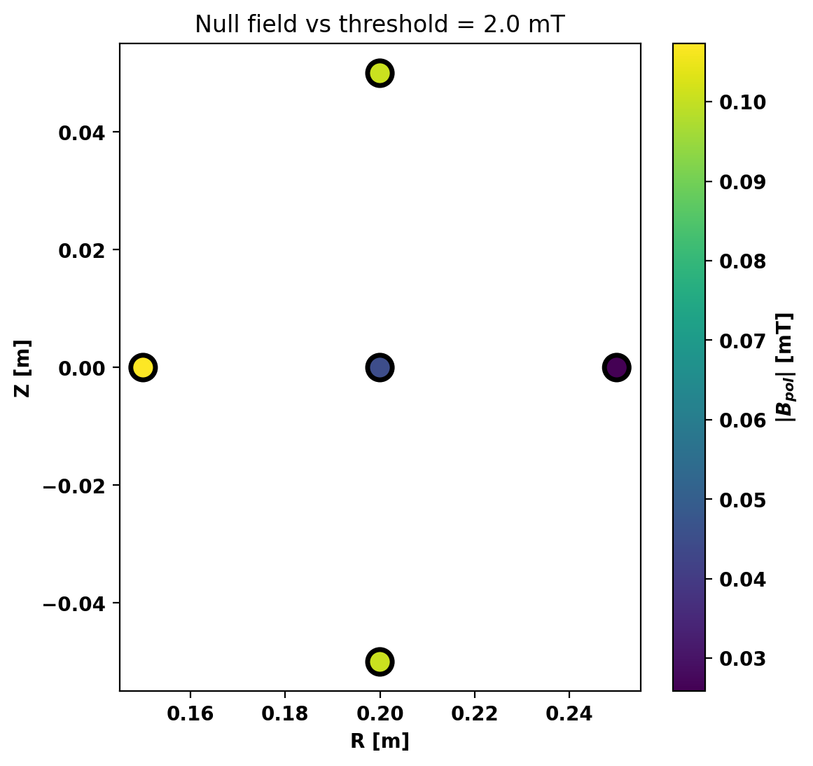
These are the residual poloidal field magnitudes \(|B_{pol}|\) at the constraint points in the null region. They set the connection length \(L_c \propto B_\phi/|B_{pol}|\) — how far a freshly-ionized electron streams along the (nearly toroidal) field before drifting into a wall. A long connection length lets electrons circulate many times and ionize enough neutral gas to start the Townsend avalanche; a stray field that is too large short-circuits that and breakdown fails.
So a good null must stay below a threshold at every point in the region, typically \(|B_{pol}| \lesssim 1\)– \(2\) mT (10–20 G). The cell below sets that threshold explicitly, checks each constraint point against it, prints a pass/fail per point, and outlines any violating point in red.
Null-field threshold check  (B_threshold = 2.00 mT):
  pt 0  R=0.200  Z=+0.000   |B_pol| =  0.045 mT   ok
  pt 1  R=0.250  Z=+0.000   |B_pol| =  0.026 mT   ok
  pt 2  R=0.150  Z=+0.000   |B_pol| =  0.107 mT   ok
  pt 3  R=0.200  Z=+0.050   |B_pol| =  0.101 mT   ok
  pt 4  R=0.200  Z=-0.050   |B_pol| =  0.101 mT   ok
=> ALL POINTS PASS
Coil current change null -> plasma
  CS01   -4.246E-04
  CS02    0.000E+00
  CS03   -8.087E-04
  CS04    0.000E+00
  CS05   -1.712E-03
  CS06    0.000E+00
  CS07   -4.132E-03
  CS08    0.000E+00
  CS09   -5.844E-01
  CS10   -5.852E-01
  CS11   -5.274E-01
  CS12   -5.302E-01
  CS13    2.060E+00
  CS14    2.064E+00
  PF01   -2.243E-01
  PF02   -1.207E+00
  PF03   -1.181E+00
  PF04   -1.624E+00
  PF05   -2.057E+00
  PF06   -2.340E+00
  PF07   -2.516E+00
  PF08   -2.519E+00
  PF09   -2.346E+00
  PF10   -2.057E+00
  PF11   -1.627E+00
  PF12   -1.191E+00
  PF13   -1.185E+00
  PF14   -1.923E-01
A small \(|B_{pol}|\) at the null is necessary but not sufficient. Whether the prefilled gas avalanches into a plasma depends on two more things:
Breakdown succeeds when the available \(E_\phi = V_{loop}/(2\pi R)\) clears \(E_{min}\) for some prefill pressure near the Paschen minimum.
max |B_pol| at null = 0.107 mT  ->  connection length L_c = 158 m
Paschen-min prefill = 2.52e-07 Torr   E_min = 0.42 V/m   (available E_phi = 0.5 V/m)
=> BREAKS DOWN
**Caveat on \(L_c\):** the factor \(0.25\) is a rough geometric constant. It makes the estimateb conservative (it under-predicts \(L_c\)): integrating an actual field line in the solved vacuum field gives a connection length several times longer. The breakdown verdict is unchanged, but treat the analytic \(L_c\) as a safe lower bound.
connection length L_c:
  analytic  0.25*a*Bphi/Bpol =    158 m
  field-line integrated      =   1016 m   (mean of 4 starts ~2 cm off-null)
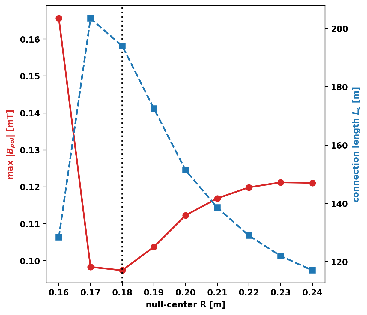
The solver already finds the coil currents that null the field at the points we ask for. The remaining design freedom is where to put the null. Below we sweep the null center in \(R\) and re-solve, looking for the location where the coils make the smallest residual \(|B_{pol}|\) (and hence the longest connection length). This is a minimal 1-D version of what could be a full \((R,Z)\) grid-scan.
Starting non-linear GS solver
     1  5.8597E-02  3.9771E-02  4.3088E-06  5.0000E-01  0.0000E+00 -0.0000E+00
     2  5.8597E-02  3.9771E-02  8.6175E-07  5.0000E-01  0.0000E+00 -0.0000E+00
 Timing:   1.0154999792575836E-002
   Source:     0.0000000000000000
   Solve:      3.3490001223981380E-003
   Boundary:   0.0000000000000000
   Other:      6.8059996701776981E-003
Starting non-linear GS solver
     1  5.8597E-02  3.9771E-02  1.8125E-06  5.0000E-01  0.0000E+00 -0.0000E+00
     2  5.8597E-02  3.9771E-02  3.6250E-07  5.0000E-01  0.0000E+00 -0.0000E+00
 Timing:   9.7640003077685833E-003
   Source:     0.0000000000000000
   Solve:      3.2509998418390751E-003
   Boundary:   0.0000000000000000
   Other:      6.5130004659295082E-003
Starting non-linear GS solver
     1  5.8597E-02  3.9771E-02  8.4874E-07  5.0000E-01  0.0000E+00 -0.0000E+00
 Timing:   5.8800000697374344E-003
   Source:     0.0000000000000000
   Solve:      1.6509997658431530E-003
   Boundary:   0.0000000000000000
   Other:      4.2290003038942814E-003
Starting non-linear GS solver
     1  5.8597E-02  3.9771E-02  9.4498E-07  5.0000E-01  0.0000E+00 -0.0000E+00
 Timing:   5.3199999965727329E-003
   Source:     0.0000000000000000
   Solve:      1.4720000326633453E-003
   Boundary:   0.0000000000000000
   Other:      3.8479999639093876E-003
Starting non-linear GS solver
     1  5.8597E-02  3.9771E-02  1.0791E-06  5.0000E-01  0.0000E+00 -0.0000E+00
     2  5.8597E-02  3.9771E-02  2.1583E-07  5.0000E-01  0.0000E+00 -0.0000E+00
 Timing:   9.7759999334812164E-003
   Source:     0.0000000000000000
   Solve:      3.1599998474121094E-003
   Boundary:   0.0000000000000000
   Other:      6.6160000860691071E-003
Starting non-linear GS solver
     1  5.8597E-02  3.9771E-02  1.0360E-06  5.0000E-01  0.0000E+00 -0.0000E+00
     2  5.8597E-02  3.9771E-02  2.0719E-07  5.0000E-01  0.0000E+00 -0.0000E+00
 Timing:   9.4190002419054508E-003
   Source:     0.0000000000000000
   Solve:      2.9840003699064255E-003
   Boundary:   0.0000000000000000
   Other:      6.4349998719990253E-003
Starting non-linear GS solver
     1  5.8597E-02  3.9771E-02  1.1228E-06  5.0000E-01  0.0000E+00 -0.0000E+00
     2  5.8597E-02  3.9771E-02  2.2456E-07  5.0000E-01  0.0000E+00 -0.0000E+00
 Timing:   9.5569998957216740E-003
   Source:     0.0000000000000000
   Solve:      3.0269999988377094E-003
   Boundary:   0.0000000000000000
   Other:      6.5299998968839645E-003
Starting non-linear GS solver
     1  5.8597E-02  3.9771E-02  1.1782E-06  5.0000E-01  0.0000E+00 -0.0000E+00
     2  5.8597E-02  3.9771E-02  2.3565E-07  5.0000E-01  0.0000E+00 -0.0000E+00
 Timing:   9.2670000158250332E-003
   Source:     0.0000000000000000
   Solve:      2.9649999924004078E-003
   Boundary:   0.0000000000000000
   Other:      6.3020000234246254E-003
Starting non-linear GS solver
     1  5.8597E-02  3.9771E-02  1.2097E-06  5.0000E-01  0.0000E+00 -0.0000E+00
     2  5.8597E-02  3.9771E-02  2.4193E-07  5.0000E-01  0.0000E+00 -0.0000E+00
 Timing:   9.6599999815225601E-003
   Source:     0.0000000000000000
   Solve:      3.0609997920691967E-003
   Boundary:   0.0000000000000000
   Other:      6.5990001894533634E-003
Cleanest null at R = 0.180 m:  |B_pol| = 0.10 mT,  L_c = 194 m
Starting non-linear GS solver
     1  5.8597E-02  3.9771E-02  4.3092E-06  5.0000E-01  0.0000E+00 -0.0000E+00
     2  5.8597E-02  3.9771E-02  8.6184E-07  5.0000E-01  0.0000E+00 -0.0000E+00
 Timing:   9.7829997539520264E-003
   Source:     0.0000000000000000
   Solve:      3.0930000357329845E-003
   Boundary:   0.0000000000000000
   Other:      6.6899997182190418E-003


/var/folders/77/9hnl3h2d5jq7v8mv35f7n_z40000gn/T/ipykernel_42417/7961170.py:11: DeprecationWarning: `set_isoflux()` is deprecated, use `set_isoflux_constraints()` instead. This function will be removed in a future version.
  mygs.set_isoflux(None)
/var/folders/77/9hnl3h2d5jq7v8mv35f7n_z40000gn/T/ipykernel_42417/7961170.py:12: DeprecationWarning: `set_saddles()` is deprecated, use `set_saddle_constraints()` instead. This function will be removed in a future version.
  mygs.set_saddles(stencil)
/var/folders/77/9hnl3h2d5jq7v8mv35f7n_z40000gn/T/ipykernel_42417/7961170.py:33: DeprecationWarning: `set_isoflux()` is deprecated, use `set_isoflux_constraints()` instead. This function will be removed in a future version.
  mygs.set_targets(); mygs.set_isoflux(None)
/var/folders/77/9hnl3h2d5jq7v8mv35f7n_z40000gn/T/ipykernel_42417/7961170.py:34: DeprecationWarning: `set_saddles()` is deprecated, use `set_saddle_constraints()` instead. This function will be removed in a future version.
  mygs.set_saddles(zero_field_pts); mygs.solve(vacuum=True)


<OpenFUSIONToolkit.TokaMaker._core.TokaMaker_equilibrium at 0x1116317c0>
The connection-length picture above has a compact engineering form that is often applied in the tokamak-startup community (from Leuer, J. A., et al. "Plasma startup design of fully superconducting tokamaks EAST and KSTAR with implications for ITER." IEEE transactions on plasma science 38.3 (2010): 333-340). Two experimentally-calibrated conditions must hold in the breakdown region:
\(\)E_\phi \ge 0.3\ \mathrm{V/m\ (ohmic)},\qquad E_\phi \ge 0.15\ \mathrm{V/m\ (ECRF\text{-}assisted)} \tag{1} \(\) \(\)\frac{E_\phi\, B_\phi}{B_T} \ge 10^3\ \mathrm{V/m} \tag{2} \(\)
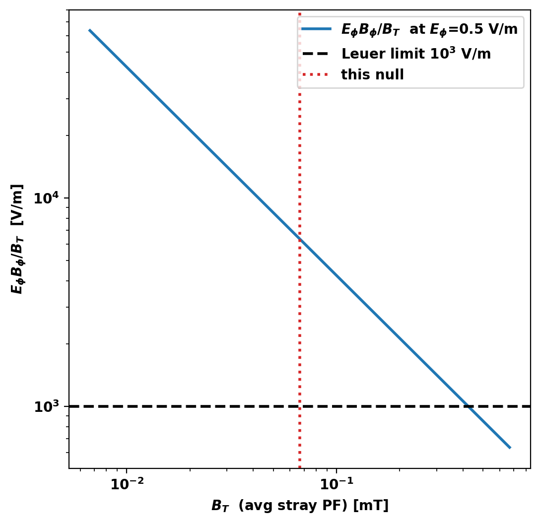
where \(E_\phi\) is the toroidal electric field (loop voltage \(V_{loop} = E_\phi\,2\pi R\)), \(B_\phi\) the toroidal field, and \(B_T\) the average stray poloidal field over the breakdown region. Criterion (2) is essentially \(E_\phi\) times the normalized connection length, since \(B_\phi/B_T \propto L_c/a\). It rewards both a strong loop voltage and a clean null at once. Below we evaluate both criteria at our null (using the same \(E_\phi\) as the Townsend/Paschen cell) and show how clean the null must be to pass (2).
Note: here \(B_T\) denotes the average stray poloidal field, computed as an area-average over the null region (not just the five constraint points, which the solver pins toward zero).
Breakdown region:   B_phi = 0.850 T    B_T (avg stray) = 0.067 mT
(1) E_phi floor:    0.30 V/m  (have 0.50)        -> OK
(2) E_phi*B_phi/B_T =    6362 V/m  (>= 1000 V/m)  -> OK
    V_loop = 0.63 V    minimum E_phi for breakdown = 0.30 V/m
 1.17.0