In this example we demonstrate how to run a time-domain simulation with current diagnostics for a simple ThinCurr model of a cylinder.

Note: Running this example requires the h5py and pyvista python packages, which are installable using pip or other standard methods.

import struct
import sys
import os
import h5py
import numpy as np
import matplotlib.pyplot as plt
import matplotlib.lines as mlines
import pyvista
pyvista.set_jupyter_backend('static') # Comment to enable interactive PyVista plots
plt.rcParams['figure.figsize']=(6,6)
plt.rcParams['font.weight']='bold'
plt.rcParams['axes.labelweight']='bold'
plt.rcParams['lines.linewidth']=2
plt.rcParams['lines.markeredgewidth']=2
%matplotlib inline
%config InlineBackend.figure_format = "retina"

Load ThinCurr library

To load the ThinCurr python module we need to tell python where to the module is located. This can be done either through the PYTHONPATH environment variable or within a script using sys.path.append() as below, where we look for the environement variable OFT_ROOTPATH to provide the path to where the OpenFUSIONToolkit is installed (/Applications/OFT for binaries on macOS).

thincurr_python_path = os.getenv('OFT_ROOTPATH')
if thincurr_python_path is not None:
    sys.path.append(os.path.join(thincurr_python_path,'python'))
from OpenFUSIONToolkit import OFT_env
from OpenFUSIONToolkit.ThinCurr import ThinCurr
from OpenFUSIONToolkit.io import histfile

Setup ThinCurr model

We now create a OFT_env instance for execution using two threads and a ThinCurr instance that utilizes that execution environment.

Once created, we setup the model from an existing HDF5 and XML mesh definition using setup_model(). For this model we have defined current jumpers using additional nodesets, which must be identified using the jumper_start argument. Here we use python-style reverse array indexing to indicate the jumpers start at the last entry in the nodeset list.

Finally, we initialize I/O for this model using setup_io() to enable output of plotting files for 3D visualization in VisIt, Paraview, or using pyvista below.

myOFT = OFT_env(nthreads=2)
tw_cyl = ThinCurr(myOFT)
tw_cyl.setup_model(mesh_file='thincurr_ex-cyl.h5',xml_filename='oft_in-jumper.xml',jumper_start=-1)
tw_cyl.setup_io()

#----------------------------------------------
Open FUSION Toolkit Initialized
Development branch:    v1_beta7
Revision id:           7aff680
Parallelization Info:
  # of MPI tasks      =    1
  # of NUMA nodes     =    1
  # of OpenMP threads =    2
Fortran input file    = /var/folders/52/n5qxh27n4w19qxzqygz2btbw0000gn/T/oft_59828/oftpyin
XML input file        = none
Integer Precisions    =    4   8
Float Precisions      =    4   8  16
Complex Precisions    =    4   8
LA backend            = native
#----------------------------------------------


Creating thin-wall model
  No V(t) driver coils found
  Loading I(t) driver coils
    Masked      0 coils from sensors
  Building holes

  Loading region resistivity:
     1  1.2570E-05

  Setup complete:
    # of points    =          782
    # of edges     =         2222
    # of cells     =         1440
    # of holes     =            1
    # of closures  =            0
    # of Vcoils    =            0
    # of Icoils    =            1

Setup sensor object

Unlike in ThinCurr Python Example: Time-domain simulation of a cylinder we are not definining any magnetic sensors. However, we must still call compute_Msensor() to setup the jumpers. During this time the orientation of positive current for each jumper is saved to a jumpers_orient.dat file in the current directory.

_, _, sensor_obj = tw_cyl.compute_Msensor()

Loading sensor information
  Setting up jumpers
Building element->sensor inductance matrix
  No magnetic sensors, skipping...
Building coil->sensor inductance matrix
  No magnetic sensors or coils, skipping...

Compute self-inductance and resistivity matrices

With the model setup, we can now compute the self-inductance and resistivity matrices. A numpy version of the self-inductance matrix will be stored at tw_plate.Lmat. By default the resistivity matrix is not moved to python as it is sparse and converting to dense representation would require an increase in memory. These matrices correspond to the \(\textrm{L}\) and \(\textrm{R}\) matrices for the physical system

\(\textrm{L} \frac{\partial I}{\partial t} + \textrm{R} I = V\)

Note: For larger models calculating the self-inductance may take some time due to the \(N^2\) interaction of the elements (see ThinCurr Python Example: Using HODLR approximation for more information).

Mc = tw_cyl.compute_Mcoil()
tw_cyl.compute_Lmat()
tw_cyl.compute_Rmat()

Building coil<->element inductance matrices
  Time =  0s          
Building element<->element self inductance matrix
  Time =  1s          
Building resistivity matrix

Run time-domain simulation

With the model fully defined we can now use run_td() to perform a time-domain simulation. In this case we simulate 80 ms using a timestep of 0.2 ms (400 steps). We also specify using a direct solver for the time-advance (direct=True) and set the current in the single I-coil defined in the XML input file as a function of time (coil_currs), where the first column specifies time points in ascending order and the remaining columns specify coil currents at each time point.

dt = 2.E-4
nsteps = 400
coil_currs = np.array([
    [0.0, 0.0],
    [2.E-2, 1.E3],
    [1.0, 1.E3]
])
tw_cyl.run_td(dt,nsteps,status_freq=10,coil_currs=coil_currs,sensor_obj=sensor_obj,direct=True)

Starting time-domain simulation
  timestep    time           sol_norm     nits    solver time
  Starting factorization
 Inverting real matrix
   Time =    1.1890000000000000E-002
      10    2.000000E-03    3.1870E-03       1        0.00
      20    4.000000E-03    6.2193E-03       1        0.00
      30    6.000000E-03    9.0309E-03       1        0.00
      40    8.000000E-03    1.1638E-02       1        0.00
      50    1.000000E-02    1.4057E-02       1        0.00
      60    1.200000E-02    1.6300E-02       1        0.00
      70    1.400000E-02    1.8380E-02       1        0.00
      80    1.600000E-02    2.0310E-02       1        0.00
      90    1.800000E-02    2.2100E-02       1        0.00
     100    2.000000E-02    2.3676E-02       1        0.00
     110    2.200000E-02    2.2037E-02       1        0.00
     120    2.400000E-02    2.0440E-02       1        0.00
     130    2.600000E-02    1.8958E-02       1        0.00
     140    2.800000E-02    1.7584E-02       1        0.00
     150    3.000000E-02    1.6310E-02       1        0.00
     160    3.200000E-02    1.5127E-02       1        0.00
     170    3.400000E-02    1.4031E-02       1        0.00
     180    3.600000E-02    1.3013E-02       1        0.00
     190    3.800000E-02    1.2070E-02       1        0.00
     200    4.000000E-02    1.1195E-02       1        0.00
     210    4.200000E-02    1.0383E-02       1        0.00
     220    4.400000E-02    9.6299E-03       1        0.00
     230    4.600000E-02    8.9316E-03       1        0.00
     240    4.800000E-02    8.2839E-03       1        0.00
     250    5.000000E-02    7.6831E-03       1        0.00
     260    5.200000E-02    7.1259E-03       1        0.00
     270    5.400000E-02    6.6091E-03       1        0.00
     280    5.600000E-02    6.1298E-03       1        0.00
     290    5.800000E-02    5.6853E-03       1        0.00
     300    6.000000E-02    5.2730E-03       1        0.00
     310    6.200000E-02    4.8905E-03       1        0.00
     320    6.400000E-02    4.5359E-03       1        0.00
     330    6.600000E-02    4.2069E-03       1        0.00
     340    6.800000E-02    3.9018E-03       1        0.00
     350    7.000000E-02    3.6188E-03       1        0.00
     360    7.200000E-02    3.3564E-03       1        0.00
     370    7.400000E-02    3.1130E-03       1        0.00
     380    7.600000E-02    2.8872E-03       1        0.00
     390    7.800000E-02    2.6778E-03       1        0.00
     400    8.000000E-02    2.4836E-03       1        0.00

Plot jumper signals

We can now plot the signals from the current jumper as a function of time. During the time-domain run this information is stored in OFT's binary history file format, which can be read using the histfile class. This class stores the resulting signals in a Python dict-like representation.

hist_file = histfile('jumpers.hist')
print(hist_file)
 
fig, ax = plt.subplots(1,1)
ax.plot(hist_file['time'],hist_file['JUMPER_0001'], label=r'$I_{Cyl}$ [A]')
ax.plot(coil_currs[:,0],2.0*coil_currs[:,1], label=r'$I_{Coil}$ [A]')
ax.legend()
ax.set_xlabel('Time [s]')
ax.set_ylabel('Jumper current [A]')
ax.set_ylim()
_ = ax.set_xlim(left=0.0,right=0.09)

OFT History file: jumpers.hist
  Number of fields = 3
  Number of entries = 401

  Fields:
    time: Simulation time [s] (d1)
    JUMPER_0001: No description (d1)
    HOLE_0001: No description (d1)

Generate plot files

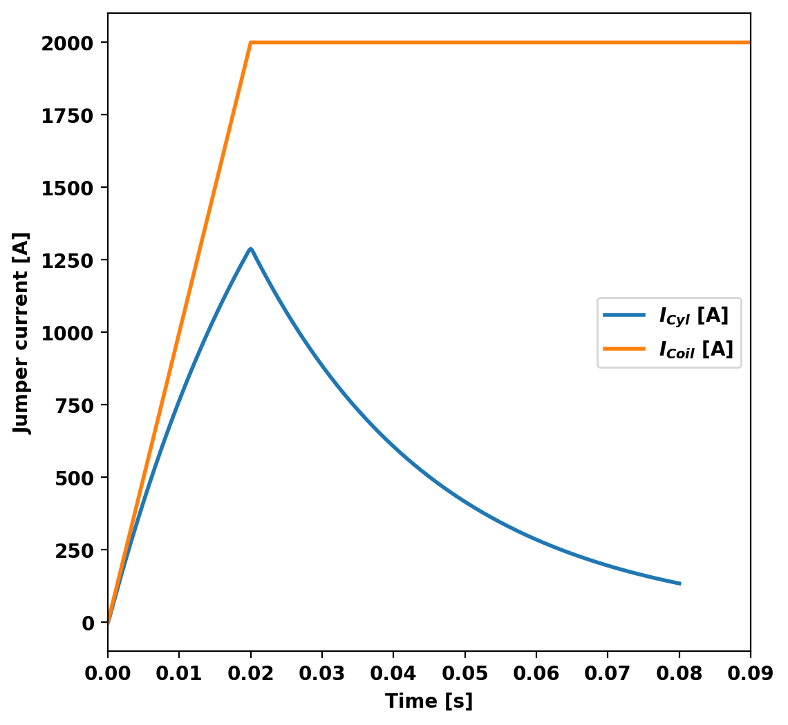
After completing the simulation we can generate plot files using plot_td(). Plot files are saved at a fixed timestep interval, specified by the nplot argument to run_td() with a default value of 10.

Once all fields have been saved for plotting build_XDMF() to generate the XDMF descriptor files for plotting with VisIt of Paraview. This method also returns a XDMF_plot_file object, which can be used to read and interact with plot data in Python (see below).

tw_cyl.plot_td(nsteps,sensor_obj=sensor_obj)

plot_data = tw_cyl.build_XDMF()

Post-processing time-domain simulation

Creating output files: oft_xdmf.XXXX.h5
  Removing old Xdmf files
    Removed 43 files
  Found Group: thincurr
    Found Mesh: icoils
      # of blocks: 1
    Found Mesh: smesh
      # of blocks: 1

Plot current fields using pyvista

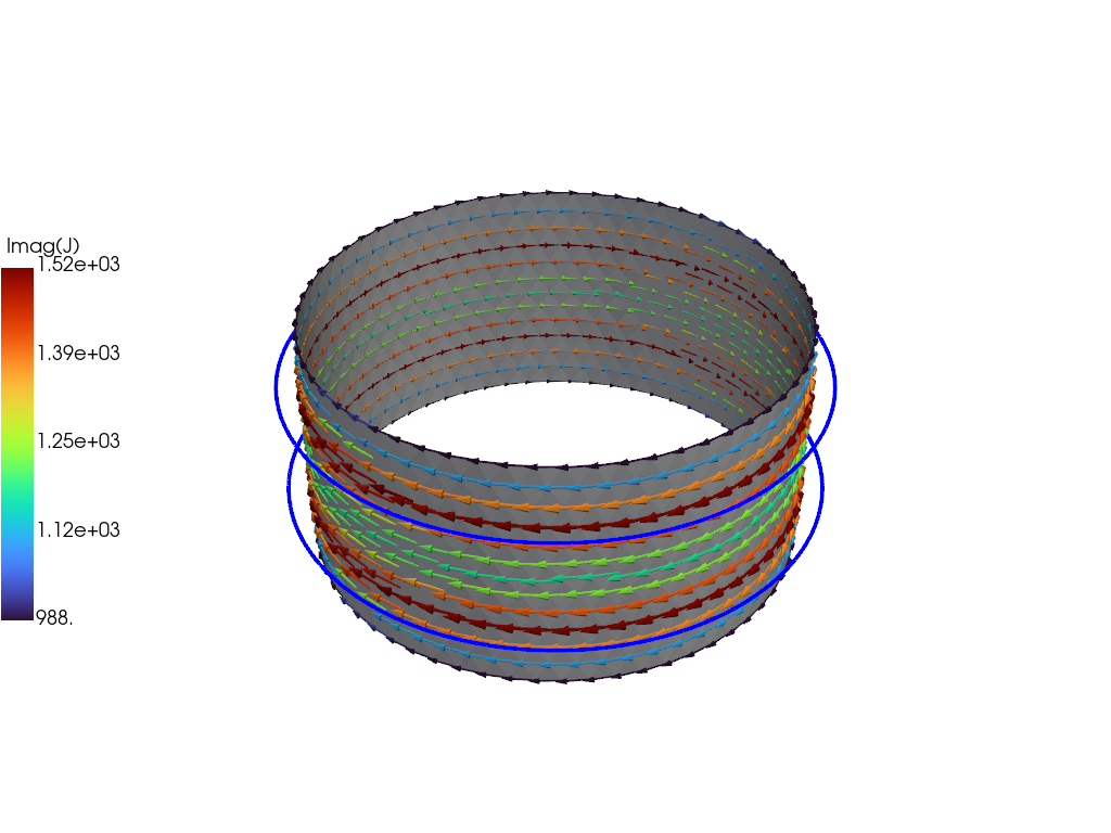
For demonstration purposes we now plot the the solution at the end of the driven phase using pyvista. We now use the plot_data object to generate a 3D plot of the current at t=2.E-2. For more information on the basic steps in this block see ThinCurr Python Example: Compute eigenstates in a plate

icoil_grid = plot_data['ThinCurr']['icoils'].get_pyvista_grid()
grid = plot_data['ThinCurr']['smesh'].get_pyvista_grid()
J = plot_data['ThinCurr']['smesh'].get_field('J_v',2.E-2)
 
# Plot mesh and current density using PyVista
p = pyvista.Plotter()
grid["vectors"] = J
grid.set_active_vectors("vectors")
scale = 0.2/(np.linalg.norm(J,axis=1)).max()
arrows = grid.glyph(scale="vectors", orient="vectors", factor=scale)
p.add_mesh(arrows, cmap="turbo", scalar_bar_args={'title': "Imag(J)", "vertical": True, "position_y":0.25, "position_x": 0.0})
p.add_mesh(grid, color="white", opacity=1.0, show_edges=False)
p.add_mesh(icoil_grid, color="blue", opacity=1.0, line_width=4)
p.show()