Running a time-dependent calculation

To run a time-dependent simulation we use similar workflow to ThinCurr Example: Eigenstates of a square plate. However, there are a couple more files to consider for most time-dependent runs. Usually in these types of simulations we are looking at the response of eddy currents to external voltages applied by currents varying in external coils or a plasma. To do this we need to define the coils (plasmas are defined using equivalent coils) and their waveforms. The coils themselves are defined in the oft_in.xmlfile as one of two types: 1.icoils: Coils that have fixed current waveforms in time 2.vcoils`: Coils have fixed voltage waveforms in time

Either type can be included or omitted separately. Within each type, constituent coils are defined by coil_set groups that can include one or more coils. For this case we have a single icoil set, composed of two circular coils (R,Z location defines the coil) with opposite polarities set by the scale attribute. More general shaped coils can also be defined by specifying a list of points defining the coil path through a npts attribute and one point per line with comma separated X,Y,Z coordinates for each point.

Current waveforms are defined in the file specified by curr_file in the thincurr_td_options options group. There is one current waveform (column) for each coil_set of the icoil type in the xml input file. The format of this file is a header line of ncols nrows followed by a series of lines where each line is a time point with the time followed by the current in each coil_set. For this case we define a current waveform that ramps from 1 kA to 0 over 100 us. Note that time points well before and after the start and end of the sequence should be provided to ensure well behaved interpolation at the end points.

With these files we can use thincurr_td to run a time-dependent simulation. Note, make sure "plot_run=F" in the "thincurr_td_options" group.

/path/to/OFT/bin/thincurr_td oft.in oft_in.xml

Contents of the input files are provided below and in the examples directory under ThinCurr/cyl, along with the necessary mesh file thincurr_ex-cyl.h5.

Post processing

Once complete you can now generate VisIt files to visualize the solution as above. First, rerun the code as above but with "plot_run=T" in the thincurr_td_options group. Once complete, you need to run the build_xdmf.py script, which generates XDMF metadata files that tells VisIt how to read the data. This can be done using the following command

python /path/to/oft/bin/build_xdmf.py

Next use VisIt to open the surf_out_XXXX.xmf database, which will contain a series timepoints with the vector field J. If you are running this example remotely and using VisIt locally you will need to copy the mesh.*.h5, scalar_dump.*.h5, vector_dump.*.h5, and *.xmf files to your local computer for visualization. The solution J at the first time point should look like the figure below.

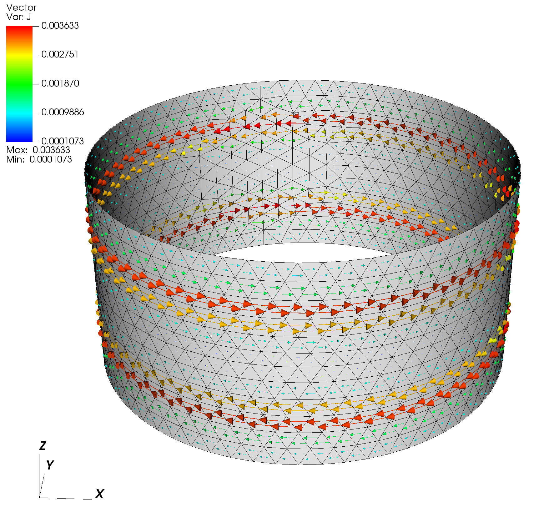
Resulting current distribution for the example time-dependent run at t=20 us

Supporting information

Input files

General global settings (oft.in)

&runtime_options
 debug=0
/

&mesh_options
 cad_type=0
/

&native_mesh_options
 filename="thincurr_ex-cyl.h5"
/

&thincurr_td_options
 curr_file='curr.drive'
 dt=2.e-5
 nsteps=200
 nplot=10
 direct=T
 save_L=F
 save_Mcoil=F
 plot_run=F
/

XML global settings (oft_in.xml)

<oft>
  <thincurr>
    <eta>1.257E-5</eta>
    <icoils>
      <coil_set>
        <coil scale="1.0">1.1, 0.25</coil>
        <coil scale="-1.0">1.1, -0.25</coil>
      </coil_set>
    </icoils>
  </thincurr>
</oft>

Coil current waveform file (curr.drive)

2 3
0.0   1.E3
1.E-4 0.0
1.0   0.0

Mesh definition

Note: For a cylinder we must define a single hole, see "Hole" elements for more information.

Cubit mesh script (thincurr_ex-cyl.jou)

reset
undo off
 
#{mesh_size=0.1}
 
# Create simple 1x1 cylinder
create curve arc radius 1 center location 0 0 0  normal 0 0 1  start angle 0 stop angle 360
sweep curve 1 vector 0 0 1  distance 1
move Surface 1 x 0 y 0 z -0.5 include_merged
 
# Generate mesh
set trimesher geometry sizing off
surface all scheme trimesh
surface all size {mesh_size}
mesh surface all
 
# Create mesh blocks
set duplicate block elements off
block 1 add surface 1
nodeset 1 add vertex 2
 
# Export grid
set large exodus file on
export Genesis  "thincurr_ex-cyl.g" overwrite block 1

The file can then be converted to OFT's native mesh format using the convert_cubit.py script as

python /path/to/OFT/bin/convert_cubit.py --in_file=thincurr_ex-cyl.g

which will yield the converted file thincurr_ex-cyl.h5.

Table of Contents

Running a time-dependent calculation

Post processing

Supporting information

Input files

Mesh definition