ThinCurr Python Example: Compute eigenstates in a plate
In this example we demonstrate how to compute eigenvalues and eigenvectors for a simple ThinCurr model.
- Note
- Running this example requires the h5py and pyvista python packages, which are installable using pip or other standard methods.
import struct
import sys
import os
import h5py
import numpy as np
import matplotlib.pyplot as plt
import matplotlib as mpl
import pyvista
plt.rcParams['figure.figsize']=(6,6)
plt.rcParams['font.weight']='bold'
plt.rcParams['axes.labelweight']='bold'
plt.rcParams['lines.linewidth']=2
plt.rcParams['lines.markeredgewidth']=2
%matplotlib inline
%config InlineBackend.figure_format = "retina"
Load ThinCurr library
To load the ThinCurr python module we need to tell python where to the module is located. This can be done either through the PYTHONPATH environment variable or within a script using sys.path.append() as below, where we look for the environement variable OFT_ROOTPATH to provide the path to where the OpenFUSIONToolkit is installed (/Applications/OFT for binaries on macOS).
thincurr_python_path = os.getenv('OFT_ROOTPATH')
if thincurr_python_path is not None:
sys.path.append(os.path.join(thincurr_python_path,'python'))
from OpenFUSIONToolkit import OFT_env
Python interface for ThinCurr thin-wall E-M functionality.
Definition __init__.py:1
Compute eigenvalues
Setup ThinCurr model
We now create a OFT_env instance for execution using two threads and a ThinCurr instance that utilizes that execution environment.
Once created, we setup the model from an existing HDF5 and XML mesh definition using setup_model().
Finally, we initialize I/O for this model using setup_io() to enable output of plotting files for 3D visualization in VisIt, Paraview, or using pyvista below.
myOFT = OFT_env(nthreads=2)
tw_plate = ThinCurr(myOFT)
tw_plate.setup_model(mesh_file='thincurr_ex-plate.h5',xml_filename='oft_in.xml')
tw_plate.setup_io()
#----------------------------------------------
Open FUSION Toolkit Initialized
Development branch:   v1_beta6
Revision id:          681e857
Parallelization Info:
  # of MPI tasks      =    1
  # of NUMA nodes     =    1
  # of OpenMP threads =    2
Fortran input file    = /var/folders/52/n5qxh27n4w19qxzqygz2btbw0000gn/T/oft_64855/oftpyin
XML input file        = none
Integer Precisions    =    4   8
Float Precisions      =    4   8  16
Complex Precisions    =    4   8
LA backend            = native
#----------------------------------------------


Creating thin-wall model
 Orientation depth =         747
  Loading V(t) driver coils
  Loading I(t) driver coils

  # of points    =          492
  # of edges     =         1393
  # of cells     =          902
  # of holes     =            0
  # of Vcoils    =            0
  # of closures  =            0
  # of Icoils    =            1

  Building holes

  Loading region resistivity:
     1  1.2570E-05
Compute self-inductance and resistivity matrices
With the model setup, we can now compute the self-inductance and resistivity matrices. A numpy version of the self-inductance matrix will be stored at tw_plate.Lmat. By default the resistivity matrix is not moved to python as it is sparse and converting to dense representation would require an increase in memory. These matrices correspond to the \(\textrm{L}\) and \(\textrm{R}\) matrices for the physical system
\(\textrm{L} \frac{\partial I}{\partial t} + \textrm{R} I = V\)
- Note
- For larger models calculating the self-inductance may take some time due to the \(N^2\) interaction of the elements (see ThinCurr Python Example: Using HODLR approximation for more information).
tw_plate.compute_Lmat()
tw_plate.compute_Rmat()
 Building element<->element self inductance matrix
     Time =  0s
 Building resistivity matrix
Compute eigenvalues/eigenvectors for the plate model
With \(\textrm{L}\) and \(\textrm{R}\) matrices we can now compute the eigenvalues and eigenvectors of the system \(\textrm{L} I = \lambda \textrm{R} I\), where the eigenvalues \(\lambda = \tau_{L/R}\) are the decay time-constants of the current distribution corresponding to each eigenvector.
eig_vals, eig_vecs = tw_plate.get_eigs(5,False)
 Starting eigenvalue solve
   Time =    3.8390000000000000E-003
 Eigenvalues
      9.7328555499775447E-003
      6.5304273569129047E-003
      6.5303149629831973E-003
      5.2500818095550300E-003
      4.7031013858612036E-003
Save data for plotting
The resulting currents can be saved for plotting using tw_plate.save_current(). Here we save each of the five eigenvectors for visualization. Once all fields have been saved for plotting tw_plate.build_XDMF() to generate the XDMF descriptor files for plotting with VisIt of Paraview. This method also returns a XDMF_plot_file object, which can be used to read and interact with plot data in Python (see below).
tw_plate.save_current(eig_vecs[0,:],'J_01')
tw_plate.save_current(eig_vecs[1,:],'J_02')
tw_plate.save_current(eig_vecs[2,:],'J_03')
tw_plate.save_current(eig_vecs[3,:],'J_04')
plot_data = tw_plate.build_XDMF()
Removing old Xdmf files
  Removed 2 files

Creating output files: oft_xdmf.XXXX.h5
  Found Group: thincurr
    Found Mesh: icoils
      # of blocks: 1
    Found Mesh: smesh
      # of blocks: 1
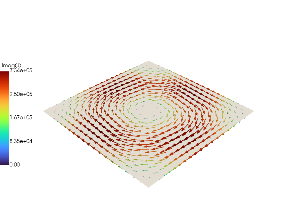
Plot current vectors on surface
Finally we plot the current vectors on the plate showing the longest-lived eddy current structure, which corresponds to a large circulation on the plate. The XDMF_plot_file class provides functionality to work with the data stored in OFT plot files, including methods to generate information for 3D plotting in Python using pyvista.
Plotting data is always associated with a specific mesh, which is itself associated with a physics group. In this case ThinCurr is the physics group and the data we are interested in is stored on the surface mesh smesh. The plot_data['ThinCurr']['smesh'] is a XDMF_plot_mesh object with further functionality for accessing data.
To plot the first eigenvector we first get the pyvista plotting grid using get_pyvista_grid() and then retrieve the vertex-centered field (J_01_v) using get_field()
grid = plot_data['ThinCurr']['smesh'].get_pyvista_grid()
J_01 = plot_data['ThinCurr']['smesh'].get_field('J_01_v')
grid["vectors"] = J_01
grid.set_active_vectors("vectors")
p = pyvista.Plotter()
scale = 0.1/(np.linalg.norm(J_01,axis=1)).max()
arrows = grid.glyph(scale="vectors", orient="vectors", factor=scale)
p.add_mesh(arrows, cmap="turbo", scalar_bar_args={'title': "Imag(J)", "vertical": True, "position_y":0.25, "position_x": 0.0})
p.add_mesh(grid, color="white", opacity=1.0, show_edges=False)
p.show(jupyter_backend='static')
Generated by