In this example we demonstrate how to build a reduced model from a large ThinCurr model and apply that model to time-domain simulations.
- Note
- Running this example requires the h5py and pyvista python packages, which are installable using
pipor other standard methods.
Load ThinCurr library
To load the ThinCurr python module we need to tell python where to the module is located. This can be done either through the PYTHONPATH environment variable or within a script using sys.path.append() as below, where we look for the environement variable OFT_ROOTPATH to provide the path to where the OpenFUSIONToolkit is installed (/Applications/OFT for binaries on macOS).
Perform time-dependen simulation with full model
Setup ThinCurr model
We now create a ThinCurr instance to use for equilibrium calculations. As this is a larger model, we use nthreads=4 to increase the number of cores used for the calculation. Once created, we setup the model from an existing HDF5 and XML mesh definition using setup_model(). We also initialize I/O for this model using setup_io() to enable output of plotting files for 3D visualization in VisIt, Paraview, or using pyvista below.
#----------------------------------------------
Open FUSION Toolkit Initialized
Development branch:   main
Revision id:          8440e61
Parallelization Info:
  Not compiled with MPI
  # of OpenMP threads =    4
Fortran input file    = oftpyin
XML input file        = none
Integer Precisions    =    4   8
Float Precisions      =    4   8  16
Complex Precisions    =    4   8
LA backend            = native
#----------------------------------------------


Creating thin-wall model
 Orientation depth =       26500
  Loading V(t) driver coils
  Loading I(t) driver coils

  # of points    =        22580
  # of edges     =        67150
  # of cells     =        44560
  # of holes     =           11
  # of Vcoils    =            0
  # of closures  =            0
  # of Icoils    =            1

  Building holes

  Loading region resistivity:
     1  1.2570E-05
Define some sensors
 Loading floop information:
   # of floops =           3
 Building element->sensor inductance matrix
 Building coil->sensor inductance matrix
Compute inductance and resistivity matrices
With the model setup, we can now compute the self-inductance matrix using HODLR. When HODLR is used the result is a pointer to the Fortran operator, which is stored at tw_torus.Lmat_hodlr. As in any other case, by default, the resistivity matrix is not moved to python as it is sparse and converting to dense representation would require an increase in memory. These matrices correspond to the \(\textrm{L}\) and \(\textrm{R}\) matrices for the physical system
\(\textrm{L} \frac{\partial I}{\partial t} + \textrm{R} I = V\)
- Note
- Even though HODLR should significantly accelerate the construction of the self-inductance matrix (see ThinCurr Example: Using HODLR approximation for more information) this process may still take some time to complete.
- The non-zero savings achieved by HODLR compression is reported after the operator is built. Where in this case only 6% of the original memory is needed resulting in a reduction from > 3 GB to ~ 230 MB (over 10x smaller)!
 Building coil<->element inductance matrices
     Time =  0s
 Building coil<->coil inductance matrix
 Partitioning grid for block low rank compressed operators
   nBlocks =                  32
   Avg block size =          686
   # of SVD =                167
   # of ACA =                161

 Building block low rank inductance operator
   Building hole and Vcoil columns
   Building diagonal blocks
     10%
     20%
     30%
     40%
     50%
     60%
     70%
     80%
     90%
   Building off-diagonal blocks using ACA+
     10%
     20%
     30%
     40%
     50%
     60%
     70%
     80%
     90%
     Compression ratio:   6.1%  ( 2.94E+07/ 4.82E+08)
     Time =  1m 49s
   Saving HODLR matrix to file: HOLDR_L.save
Building resistivity matrix
Compute eigenvalues/eigenvectors for the plate model
With \(\textrm{L}\) and \(\textrm{R}\) matrices we can now compute the eigenvalues and eigenvectors of the system \(\textrm{L} I = \lambda \textrm{R} I\), where the eigenvalues \(\lambda = \tau_{L/R}\) are the decay time-constants of the current distribution corresponding to each eigenvector.
 Starting eigenvalue solve
   Time =    3.1751179999999999
 Eigenvalues
      3.8803528411153393E-002
      2.3122417445974628E-002
      2.3121318885336407E-002
      2.1444721888242122E-002
      2.0605569150466851E-002
Run time-domain simulation
 Starting simulation
 Timestep           10   2.00000009E-03   22.7324581              32
 Timestep           20   4.00000019E-03   44.1192436              18
 Timestep           30   6.00000005E-03   42.2027016              32
 Timestep           40   8.00000038E-03   39.9049377              32
 Timestep           50   9.99999978E-03   37.7692757              32
 Timestep           60   1.20000001E-02   35.7698631              32
 Timestep           70   1.40000004E-02   33.8907852              32
 Timestep           80   1.60000008E-02   32.1206093              32
 Timestep           90   1.79999992E-02   30.4503746              32
 Timestep          100   1.99999996E-02   28.8726807              32
 Timestep          110   2.19999999E-02   27.3811455              32
 Timestep          120   2.40000002E-02   25.9701900              32
 Timestep          130   2.60000005E-02   24.6347961              32
 Timestep          140   2.80000009E-02   23.3704243              32
 Timestep          150   2.99999993E-02   22.1729164              32
 Timestep          160   3.20000015E-02   21.0384293              32
 Timestep          170   3.40000018E-02   19.9634075              32
 Timestep          180   3.59999985E-02   18.9445362              32
 Timestep          190   3.79999988E-02   17.9787235              32
 Timestep          200   3.99999991E-02   17.0630703              32
Compute B-field reconstruction operator
 Building block low rank magnetic field operator
   Building hole and Vcoil columns
   Building diagonal blocks
     10%
     20%
     30%
     40%
     50%
     60%
     70%
     80%
     90%
   Building off-diagonal blocks using ACA+
     10%
     20%
     30%
     40%
     50%
     60%
     70%
     80%
     90%
     Compression ratio:   7.1%  ( 1.06E+08/ 1.49E+09)
     Time =  3m 33s
   Saving HODLR matrix from file: HODLR_B.save
Generate plot files from run
 Post-processing simulation
Removing old Xdmf files
Creating output files
Load sensor signals from time-domain run
OFT History file: floops.hist
  Number of fields = 4
  Number of entries = 201

  Fields:
    time: Simulation time [s] (d1)
    Bz_1: No description (d1)
    Bz_2: No description (d1)
    Bz_3: No description (d1)
Build PyVista information for plotting
Explicit model reduction
In addition to HODLR, we can also explicitly reduce the model's size by projecting onto a fixed set of current strucutures using build_reduced_model(). In this case we use the 25 eigenvalues computed above, which will result in a system that reasonably matches slow dynamics with characterisitic times longer than the fastest eigenvalue.
- Note
- We have now reduced our system to only 160 KB from > 3 GB (over 18,000x smaller)! Assuming we are only interested in slow dynamics of course.
Compute and compare eigenvalues
After building the reduced system was can compare the eigenvalues of the original system to show that the characteristic timescales are maintained.
  Reduced      Original     (% Error )
  3.8804E+01   3.8804E+01   (4.32E-09)
  2.3122E+01   2.3122E+01   (2.14E-09)
  2.3121E+01   2.3121E+01   (1.09E-09)
  2.1445E+01   2.1445E+01   (1.91E-08)
  2.0606E+01   2.0606E+01   (1.20E-09)
   ...          ...          ...
  1.8735E+01   1.8735E+01   (4.90E-09)
  5.7417E+00   5.7417E+00   (3.01E-09)
  5.6741E+00   5.6741E+00   (2.51E-09)
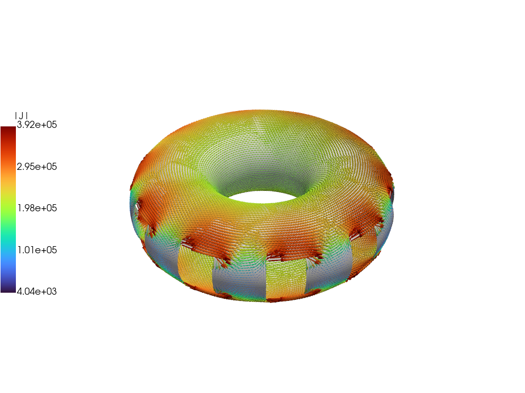
Compare current distributions
We can also plot the current distributions for the eigenmodes to show that they have the same structure as the original model.
Run time-dependent simulation
Timestep 0   0.0000E+00   0.0000E+00
Timestep 10   2.0000E-03   3.1344E+00
Timestep 20   4.0000E-03   6.0592E+00
Timestep 30   6.0000E-03   5.7573E+00
Timestep 40   8.0000E-03   5.4154E+00
Timestep 50   1.0000E-02   5.1068E+00
Timestep 60   1.2000E-02   4.8245E+00
Timestep 70   1.4000E-02   4.5637E+00
Timestep 80   1.6000E-02   4.3210E+00
Timestep 90   1.8000E-02   4.0941E+00
Timestep 100   2.0000E-02   3.8811E+00
Timestep 110   2.2000E-02   3.6806E+00
Timestep 120   2.4000E-02   3.4915E+00
Timestep 130   2.6000E-02   3.3129E+00
Timestep 140   2.8000E-02   3.1440E+00
Timestep 150   3.0000E-02   2.9841E+00
Timestep 160   3.2000E-02   2.8327E+00
Timestep 170   3.4000E-02   2.6892E+00
Timestep 180   3.6000E-02   2.5531E+00
Timestep 190   3.8000E-02   2.4241E+00
Timestep 200   4.0000E-02   2.3017E+00
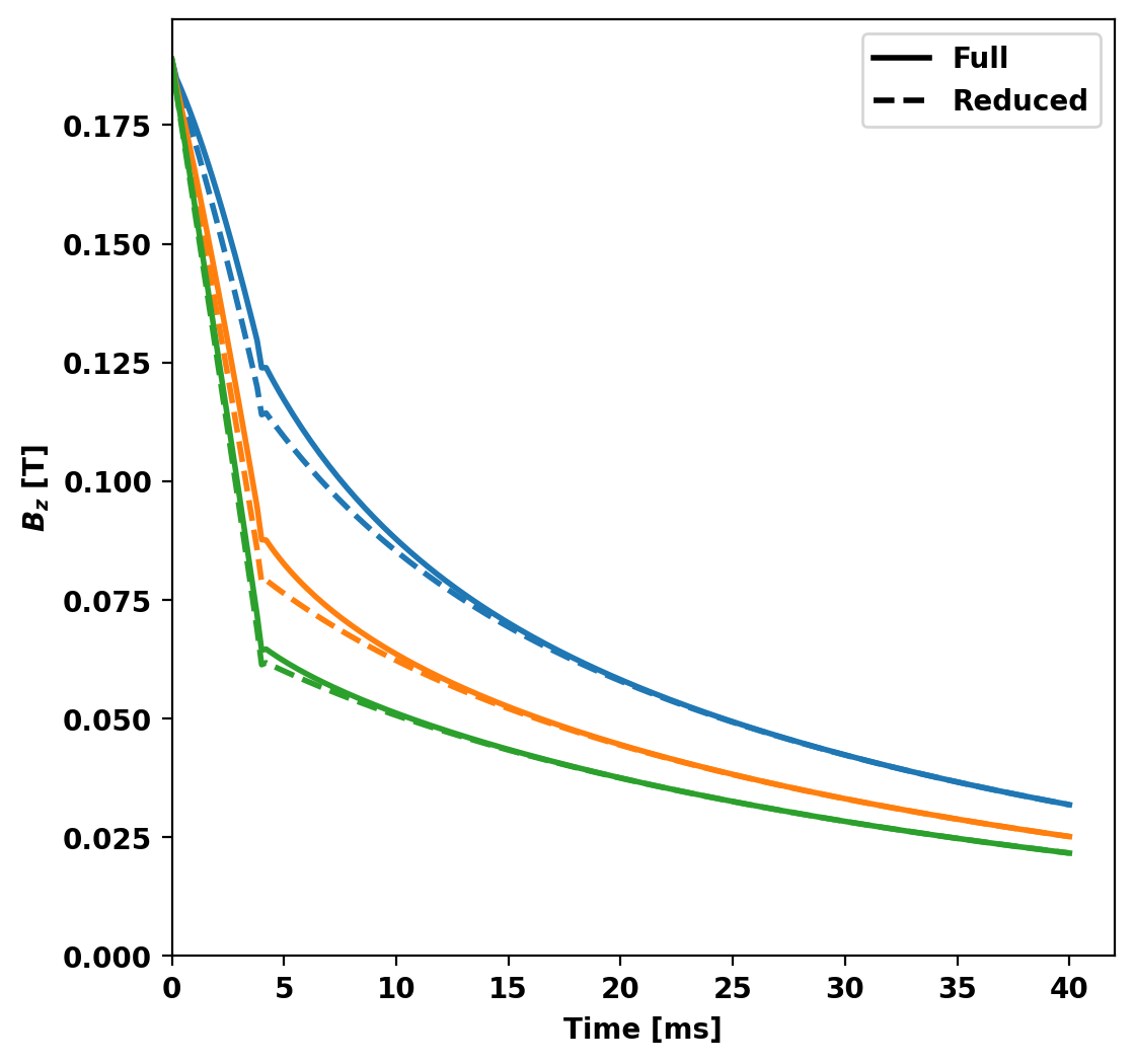
Compare sensor signals
Now we compare the probe signals from full and reduced models, noting good agreement overall with some discrepancy early in time with the results converging at later times.
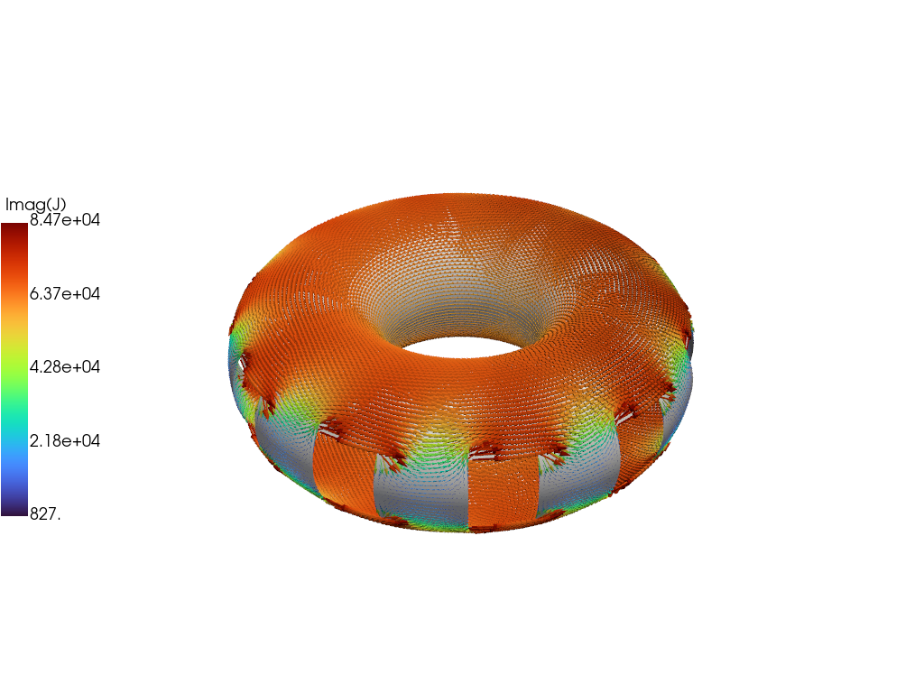
Compare current distribution
We can plot the current distributions for the eigenmodes to show that they have nearly the same structure and time-dependence as the full model. Below comparison is performed at \(t = 20\) ms showing good agreement, which should only improve at later times.
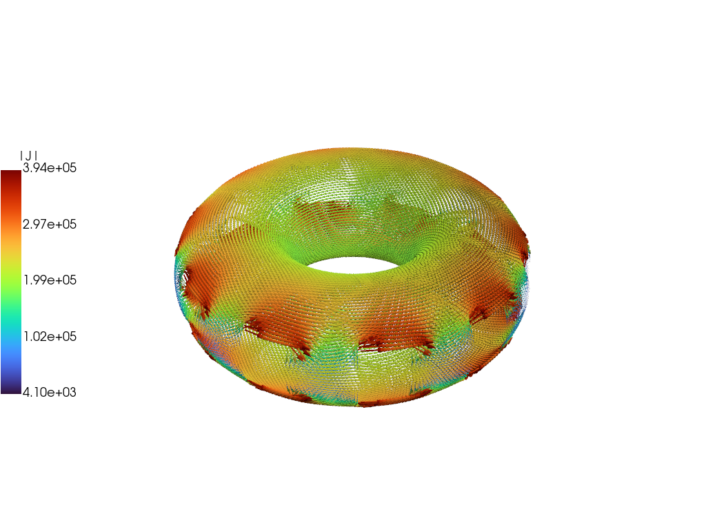
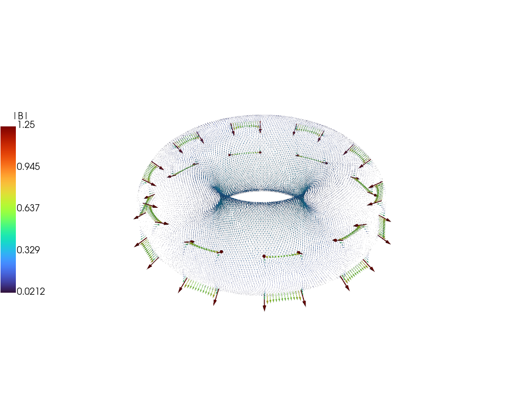
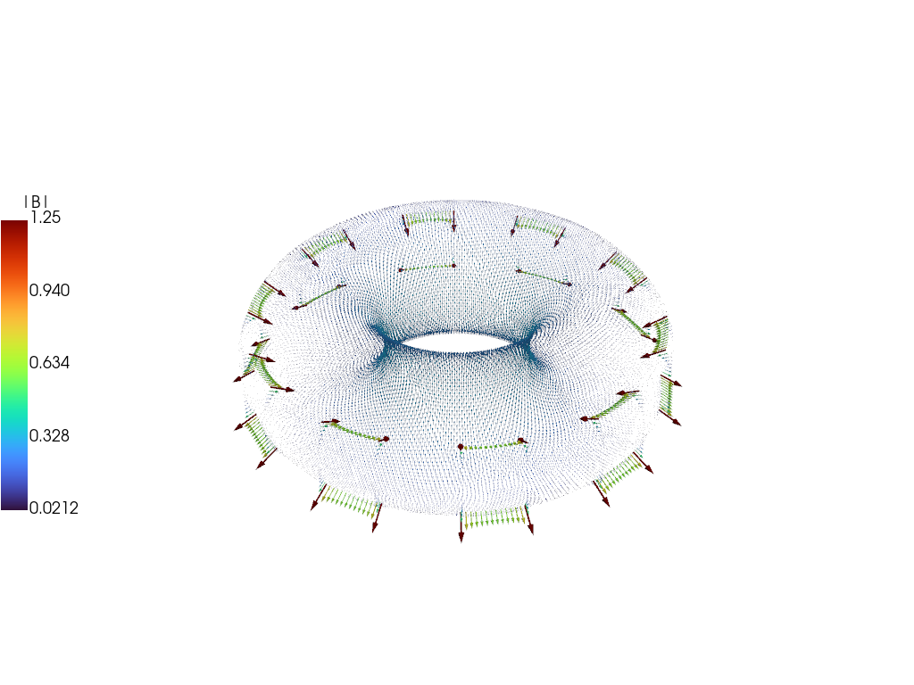
Compare magnetic field
As with the current we can also compare the magnetic field between the full simulation and the reduced model, showing excellent visual agreement at \(t = 20\) ms.
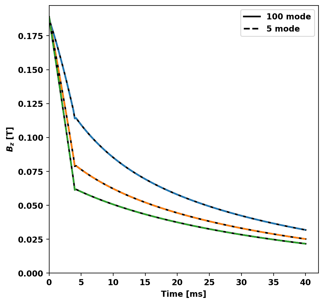
Further model reduction
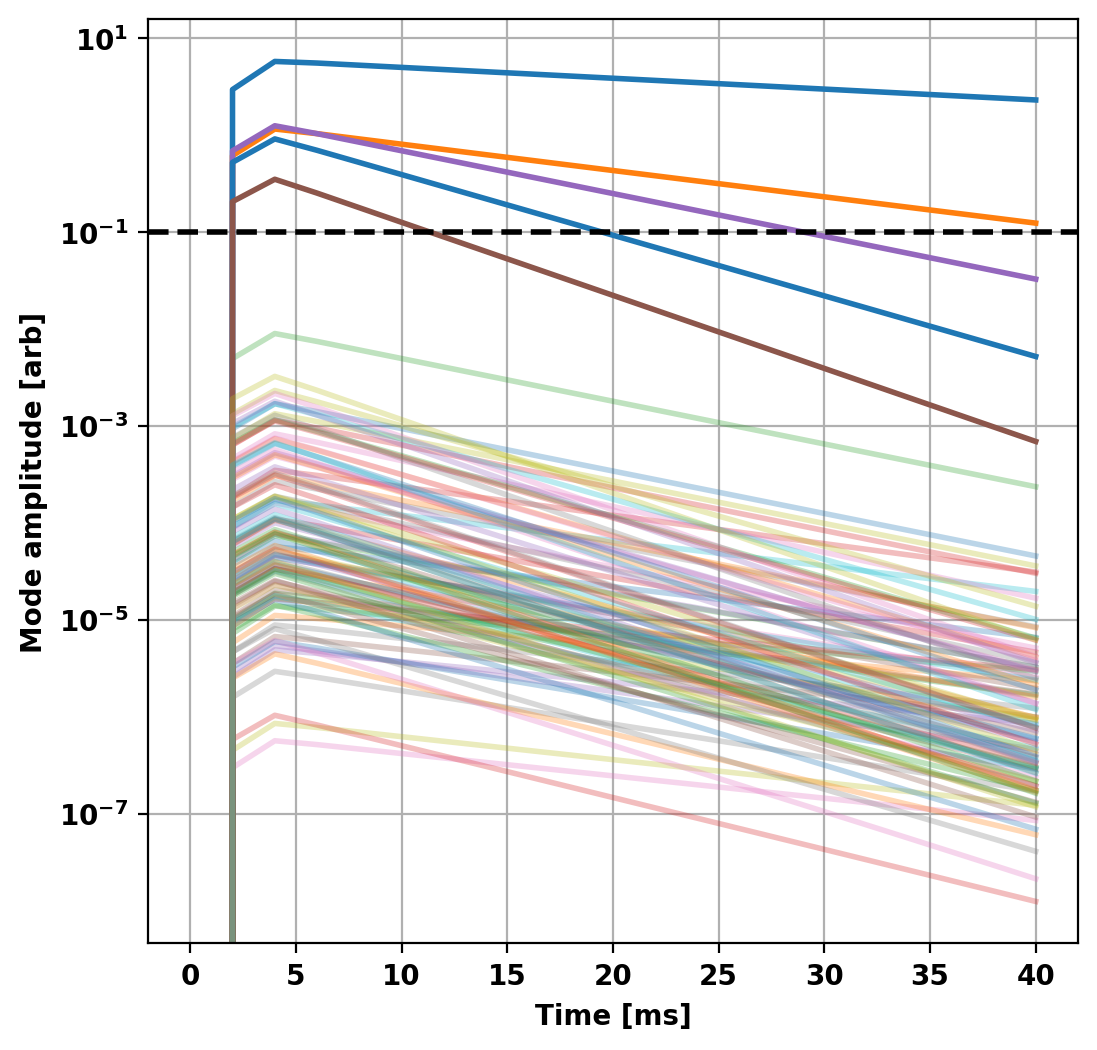
Determine most active modes
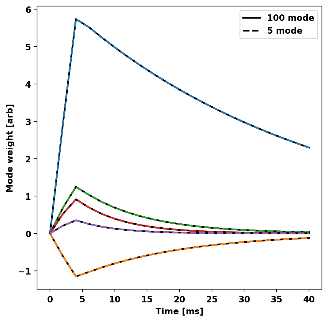
To further reduce the model we can look at the output of the previous to determine which modes in the basis set are active in the chosen simulation. In this case, the vast majority of the energy in the system is contained in only the first 5 modes.
This makes sense as all the sources driving our system are axisymmetric (single circular current filament) and as a result we expect all the eigenstructures with toroidal mode number greater than zero to have very little coupling to this structure (ideally zero). Additionally, as the L/R system results in orthogonal eigenvectors we don't expect any coupling between modes themselves. This can be seen as all modes decay exponentially (linear on semilog plot) after the driving voltage drops to zero.
Repeat calculations with minimal model
We now repeat the eigenvalue and time-domain solves from above with the further reduced model.
- Note
- We have now reduced our system to only 200 Bytes from > 3 GB (15,000,000x smaller)! Assuming we are only interested in axisymmetric slow dynamics of course.
Compute and compare eigenvalues
  Reduced      Original     (% Error )
  3.8804E+01   3.8804E+01   (4.32E-09)
  1.6008E+01   1.6008E+01   (2.66E-09)
  9.8463E+00   9.8463E+00   (1.84E-09)
  6.9472E+00   6.9472E+00   (1.86E-09)
  5.7673E+00   5.7673E+00   (7.25E-10)
Run time-dependent simulation
Timestep 0   0.0000E+00   0.0000E+00
Timestep 10   2.0000E-03   3.1344E+00
Timestep 20   4.0000E-03   6.0592E+00
Timestep 30   6.0000E-03   5.7573E+00
Timestep 40   8.0000E-03   5.4154E+00
Timestep 50   1.0000E-02   5.1068E+00
Timestep 60   1.2000E-02   4.8245E+00
Timestep 70   1.4000E-02   4.5637E+00
Timestep 80   1.6000E-02   4.3210E+00
Timestep 90   1.8000E-02   4.0941E+00
Timestep 100   2.0000E-02   3.8811E+00
Timestep 110   2.2000E-02   3.6806E+00
Timestep 120   2.4000E-02   3.4915E+00
Timestep 130   2.6000E-02   3.3129E+00
Timestep 140   2.8000E-02   3.1440E+00
Timestep 150   3.0000E-02   2.9841E+00
Timestep 160   3.2000E-02   2.8327E+00
Timestep 170   3.4000E-02   2.6892E+00
Timestep 180   3.6000E-02   2.5531E+00
Timestep 190   3.8000E-02   2.4241E+00
Timestep 200   4.0000E-02   2.3017E+00
Compare reduced models
First we compare the amplitude of each component (basis weight) of the two reduced models in time to show that they have the same behavior even with fewer modes in the system.
Now we compare the probe signals from the two reduced models showing that the results overlay eachother.