TokaMaker Meshing Example: Building an LDX-like mesh

In this example we show how to generate a mesh for an LDX-like levitated dipole using TokaMaker's built in mesh generation.

Warning

Dipole equilibrium support is still in development. Please be careful when using this feature and report any issues.

Note

Running this example requires the h5py python packages, which is installable using pip or other standard methods.

import os
import sys
import json
import numpy as np
import matplotlib.pyplot as plt
plt.rcParams['figure.figsize']=(6,6)
plt.rcParams['font.weight']='bold'
plt.rcParams['axes.labelweight']='bold'
plt.rcParams['lines.linewidth']=2
plt.rcParams['lines.markeredgewidth']=2
%matplotlib inline
%config InlineBackend.figure_format = "retina"

Load TokaMaker library

To load the TokaMaker python module we need to tell python where to the module is located. This can be done either through the PYTHONPATH environment variable or using within a script using sys.path.append() as below, where we look for the environement variable OFT_ROOTPATH to provide the path to where the OpenFUSIONToolkit is installed (/Applications/OFT on macOS).

For meshing we will use the gs_Domain class to build a 2D triangular grid suitable for Grad-Shafranov equilibria. This class uses the triangle code through a simple internal python wrapper within OFT.

tokamaker_python_path = os.getenv('OFT_ROOTPATH')
if tokamaker_python_path is not None:
    sys.path.append(os.path.join(tokamaker_python_path,'python'))
from OpenFUSIONToolkit.TokaMaker.meshing import gs_Domain, save_gs_mesh

Build mesh

Set mesh resolution for each region

First we define some target sizes to set the resolution in our grid. These variables will be used later and represent the target edge size within a given region, where units are in meters.

Note

When setting up a new machine these values will need to scale with the overall size of the device/domain. Additionally, one should perform a convergence study, by increasing resolution (decreasing target size) by at least a factor of two in all regions to ensure the results are not sensitive to your choice of grid size.

plasma_dx = 0.05
coil_dx = 0.02
vv_dx = 0.02
vac_dx = 0.12

Define regions and attributes

We now create and define the various logical mesh regions. In the dipole case we have 4 region groups:

• air: The region outside the vacuum vessel
• plasma: The region inside the limiter (vacuum vessel) where the plasma will exist
• vv: The vacuum vessel
• vacuum: The vacuum region inside the floating coil cryostat
• fcoil, lcoil: The Dipole (floating) and levitation coils

For each region you can provide a target size and one of four region types:

• plasma: The region where the plasma can exist and the classic Grad-Shafranov equation with \(F*F'\) and \(P'\) are allowed. There can only be one region of this type
• vacuum: A region where no current can flow and \(\nabla^* \psi = 0\) is solved
• boundary: A special case of the vacuum region, which forms the outer boundary of the computational domain. A region of this type is required if more than one region is specified
• conductor: A region where toroidal current can flow passively (no externally applied voltage). For this type of region the resistivity should be specified with the argument eta in units of \(\omega \mathrm{-m}\).
• coil: A region where toroidal current can flow with specified amplitude through set_coil_currents() or via shape optimization set_coil_reg() and set_isoflux()

Note

For a dipole we also we the inner_limiter argument to true for the vacuum region to mark it as the inner limiter.

# Create a G-S domain
gs_mesh = gs_Domain()
# Define region information for mesh
gs_mesh.define_region('air',vac_dx,'boundary')                         # Define the bounding region
gs_mesh.define_region('plasma1',plasma_dx,'plasma')                    # Define the main plasma region and resolution
gs_mesh.define_region('plasma2',plasma_dx*0.5,'plasma')                # Define a packed plasma region and resolution
gs_mesh.define_region('vacuum',plasma_dx,'vacuum',inner_limiter=True)  # Define the vacuum inside the cryostat
gs_mesh.define_region('vv',vv_dx,'conductor',eta=1.E-5)                # Define the VV
 
gs_mesh.define_region('fcoil',coil_dx,'coil',nTurns=716)               # Define the dipole coil (fcoil)
gs_mesh.define_region('lcoil',coil_dx,'coil',nTurns=2800)              # Define the levitation coil (lcoil)

Define geometry for region boundaries

Once the region types and properties are defined we now define the geometry of the mesh using shapes and references to the defined regions.

First, we set some geometry values that approximate the LDX device based on D.T. Garnier et al., Fusion Eng. Des. (2006).

vv_width = 2.5                   # Outer radius of VV
vv_inner_height = 2.4/2.08*2.5   # Height at center of VV
vv_outer_height = 1.18/2.08*2.5  # Height at outside of VV
vv_thickness = 0.02              # Thickness of VV
 
lcoil_height = 0.05/2.08*2.5     # Height of Lcoil
lcoil_inner = 0.410/2.0          # Lcoil inner radius
lcoil_outer = 1.32/2.0           # Lcoil outer radius
lcoil_z = 1.61                   # Lcoil vertical position

Once the region types and properties are defined we now define the geometry of the mesh using shapes and references to the defined regions.

1. The plasma region is defined by marking a location in this region
2. As the VV goes all the way to the geometric axis we need to define the boundary region explicitly so that the intersection points are present in both the VV and boundary contours.
3. The vacuum vessel is then added as a "polygon" with curves defining the inner and outer edges respectively.
4. The inner coil case/limiter is defined as a simple circular path
5. The dipole is defined using the outline from D.T. Garnier et al.
6. The levitation coil is defined as simple rectangles

# Define plasma region by location
gs_mesh.add_enclosed([1.7,0.0],'plasma1')
# Define higher resolution region
gs_mesh.add_rectangle(0.75,0.0,1.5,1.0,'plasma2',parent_name='plasma1')
 
# Define outer boundary path with points at the VV intersection
boundary_path = np.array([
    [0.0,            0.5],
    [0.0,            vv_inner_height/2.0],
    [0.0,            vv_inner_height/2.0+vv_thickness],
    [0.0,           (lcoil_z+lcoil_height)*1.3],
    [vv_width*1.3,  (lcoil_z+lcoil_height)*1.3],
    [vv_width*1.3, -(lcoil_z+lcoil_height)*1.3],
    [0.0,          -(lcoil_z+lcoil_height)*1.3],
    [0.0,          -(vv_inner_height/2.0+vv_thickness)],
    [0.0,          - vv_inner_height/2.0],
    [0.0,          -0.5]
])
gs_mesh.add_polygon(boundary_path,'air')
 
# Define VV geometry
vv_inner = np.array([
    [0.0,             -vv_inner_height/2.0],
    [lcoil_outer*1.2, -vv_inner_height/2.0],
    [vv_width,        -vv_outer_height/2.0],
    [vv_width,         vv_outer_height/2.0],
    [lcoil_outer*1.2,  vv_inner_height/2.0],
    [0.0,              vv_inner_height/2.0]
])
vv_outer = np.array([
    [0.0,                     vv_inner_height/2.0+vv_thickness],
    [lcoil_outer*1.2,         vv_inner_height/2.0+vv_thickness],
    [vv_width+vv_thickness,   vv_outer_height/2.0+vv_thickness],
    [vv_width+vv_thickness, -(vv_outer_height/2.0+vv_thickness)],
    [lcoil_outer*1.2,       -(vv_inner_height/2.0+vv_thickness)],
    [0.0,                   -(vv_inner_height/2.0+vv_thickness)]
])
gs_mesh.add_polygon(np.vstack((vv_inner,vv_outer)),'vv',parent_name='air')
 
# Define cryostat case
theta = np.linspace(0.0,2.0*np.pi,100,endpoint=False)
r1 = 0.445/2.0; r2 = 1.14/2.0
dipole_case = np.vstack((
    (r2-r1)*np.cos(theta)/2.0+(r2+r1)/2.0,
    (r2-r1)*np.sin(theta)/2.0,
)).transpose()
gs_mesh.add_polygon(dipole_case,'vacuum',parent_name='plasma2')
 
# Define Fcoil dimensions (simplified to remove innermost windings)
fcoil_outline = np.array([
    [0.555/2.0, 0.125/2.0],
    [0.585/2.0, 0.125/2.0],
    [0.585/2.0, 0.162/2.0],
    [0.764/2.0, 0.162/2.0],
    [0.764/2.0, -0.162/2.0],
    [0.585/2.0, -0.162/2.0],
    [0.585/2.0, -0.125/2.0],
    [0.555/2.0, -0.125/2.0]
])
gs_mesh.add_polygon(fcoil_outline,'fcoil',parent_name='vacuum')
 
# Define Lcoil
gs_mesh.add_rectangle((lcoil_inner+lcoil_outer)/2.0,lcoil_z,(lcoil_outer-lcoil_inner),lcoil_height,'lcoil',parent_name='air')

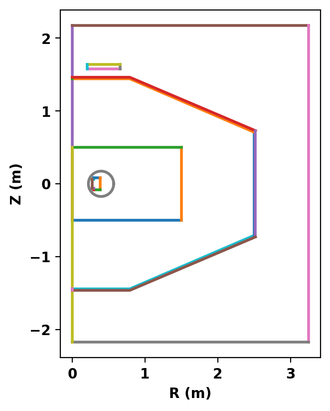
Plot topology

After defining the logical and physical topology we can now plot the curves within the definitions to double check everything is in the right place.

fig, ax = plt.subplots(1,1,figsize=(4,4),constrained_layout=True)
gs_mesh.plot_topology(fig,ax)

Create mesh

Now we generate the actual mesh using the build_mesh() method. Additionally, if coil and/or conductor regions are defined the get_coils() and get_conductors() methods should also be called to get descriptive dictionaries for later use in TokaMaker. This step may take a few moments as triangle generates the mesh.

Note that, as is common with unstructured meshes, the mesh is stored a list of points mesh_pts of size (np,2), a list of cells formed from three points each mesh_lc of size (nc,3), and an array providing a region id number for each cell mesh_reg of size (nc,), which is mapped to the names above using the coil_dict and cond_dict dictionaries.

mesh_pts, mesh_lc, mesh_reg = gs_mesh.build_mesh()
coil_dict = gs_mesh.get_coils()
cond_dict = gs_mesh.get_conductors()

Assembling regions:
  # of unique points    = 1104
  # of unique segments  = 32
Generating mesh:
  # of points  = 8546
  # of cells   = 16912
  # of regions = 6

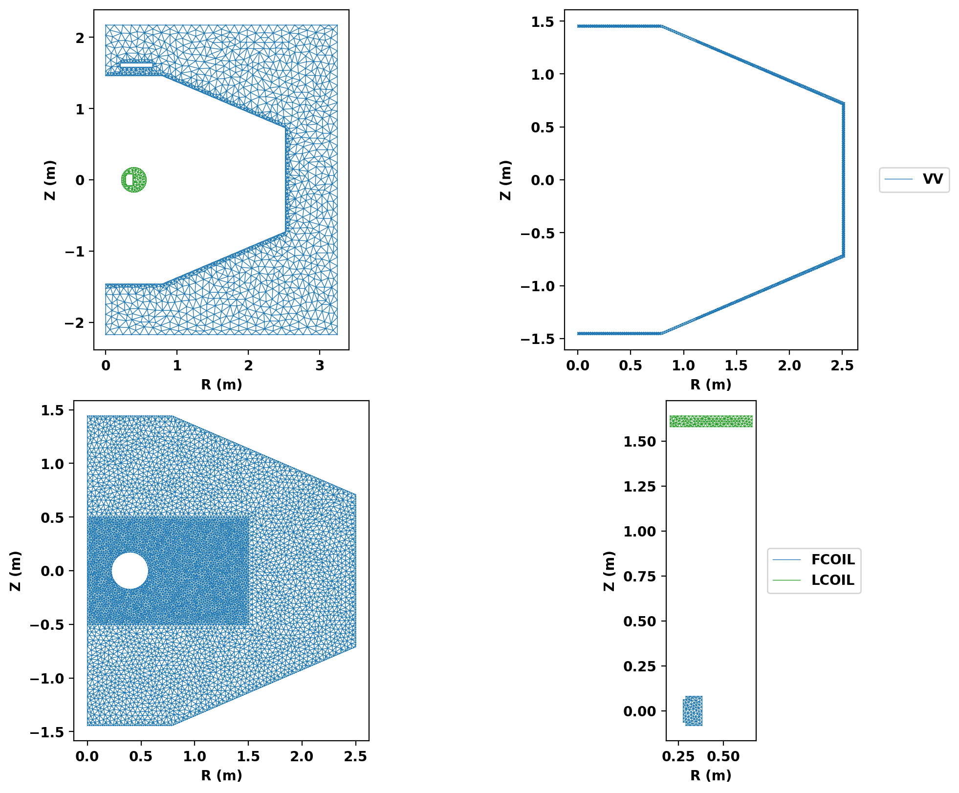
Plot resulting regions and grid

We now plot the mesh by region to inspect proper generation.

fig, ax = plt.subplots(2,2,figsize=(10,8),constrained_layout=True)
gs_mesh.plot_mesh(fig,ax)

Save mesh for later use

As generation of the mesh often takes comparable, or longer, time compare to runs in TokaMaker it is useful to separate generation of the mesh into a different script as demonstrated here. The method save_gs_mesh() can be used to save the resulting information for later use. This is done using and an HDF5 file through the h5py library.

save_gs_mesh(mesh_pts,mesh_lc,mesh_reg,coil_dict,cond_dict,'dipole_mesh.h5')