In this example we demonstrate:

1) How to reproduce a DIII-D equilibrium using an inverse solve from EFIT by reading in inputs from a gEQDSK file. 2) How to reproduce a DIII-D equilibrium using an forward solve from EFIT by reading in inputs from a gEQDSK file. 3) How to compute linear growth rates and perform time-dependent simulation of a Vertical Displacement Event (VDE) using this equilibrium

This example utilizes the mesh built in TokaMaker Meshing Example: Building a mesh for DIII-D.

Note: Running this example requires the h5py python package, which is installable using pip or other standard methods.

import os
import sys
import numpy as np
import matplotlib.pyplot as plt
plt.rcParams['figure.figsize']=(6,6)
plt.rcParams['font.weight']='bold'
plt.rcParams['axes.labelweight']='bold'
plt.rcParams['lines.linewidth']=2
plt.rcParams['lines.markeredgewidth']=2
%matplotlib inline
%config InlineBackend.figure_format = "retina"

Load TokaMaker library

To load the TokaMaker python module we need to tell python where to the module is located. This can be done either through the PYTHONPATH environment variable or using within a script using sys.path.append() as below, where we look for the environement variable OFT_ROOTPATH to provide the path to where the OpenFUSIONToolkit is installed (/Applications/OFT on macOS).

tokamaker_python_path = os.getenv('OFT_ROOTPATH')
if tokamaker_python_path is not None:
    sys.path.append(os.path.join(tokamaker_python_path,'python'))
from OpenFUSIONToolkit import OFT_env
from OpenFUSIONToolkit.TokaMaker import TokaMaker
from OpenFUSIONToolkit.TokaMaker.meshing import load_gs_mesh
from OpenFUSIONToolkit.TokaMaker.util import create_isoflux, read_eqdsk

Read equilibrium from gEQDSK file

A dictionary containing the equilibrium information is obtained using read_eqdsk(). The dictionary contains multiple key quantities that are useful for reproducing the equilibrium in TokaMaker:

eqdsk['rcentr']: The R coordinate of the plasma center
eqdsk['bcentr']: The magnetic field at the plasma center
eqdsk['ip']: Total plasma current
eqdsk['pres']: Pressure profile
eqdsk['pprime']: P' profile
eqdsk['ffprim']: F*F' profile
eqdsk['rzout']: RZ coordinates of the last closed flux surface

eqdsk = read_eqdsk('g192185.02440')

Compute equilibria

Initialize TokaMaker object

We now create a OFT_env instance for execution using two threads and a TokaMaker instance to use for equilibrium calculations. Note at present only a single TokaMaker instance can be used per python kernel, so this command should only be called once in a given Jupyter notebook or python script. In the future this restriction may be relaxed.

myOFT = OFT_env(nthreads=2)

mygs = TokaMaker(myOFT)

#----------------------------------------------
Open FUSION Toolkit Initialized
Development branch:   v1_beta6
Revision id:          681e857
Parallelization Info:
  # of MPI tasks      =    1
  # of NUMA nodes     =    1
  # of OpenMP threads =    2
Fortran input file    = /var/folders/52/n5qxh27n4w19qxzqygz2btbw0000gn/T/oft_64612/oftpyin
XML input file        = none
Integer Precisions    =    4   8
Float Precisions      =    4   8  16
Complex Precisions    =    4   8
LA backend            = native
#----------------------------------------------

Update default settings

Sometimes it is useful to modify the default TokaMaker settings. Here we update one setting to help with convergence:

mygs.settings.maxits: This sets the maximum non-linear iteration count for G-S solver, and should often be increased from the default setting of 40 iterations.

Settings can be modified before running setup() or at any time during execution by adjusting desired values and then calling update_settings().

mygs.settings.maxits = 200

Load mesh into TokaMaker

Now we load the mesh generated in TokaMaker Meshing Example: Building a mesh for DIII-D using load_gs_mesh() and setup_mesh. Then we use setup_regions(), passing the conductor and coil dictionaries for the mesh, to define the different region types. Finally, we call setup() to setup the required solver objects. During this call we can specify the desired element order (min=2, max=4) and the toroidal field through F0 = B0*R0, where B0 is the toroidal field at a reference location R0.

mesh_pts,mesh_lc,mesh_reg,coil_dict,cond_dict = load_gs_mesh('DIIID_mesh.h5')
mygs.setup_mesh(mesh_pts, mesh_lc, mesh_reg)
mygs.setup_regions(cond_dict=cond_dict,coil_dict=coil_dict)
mygs.setup(order=2,F0=eqdsk['rcentr']*eqdsk['bcentr'])

**** Loading OFT surface mesh

**** Generating surface grid level  1
  Generating boundary domain linkage
  Mesh statistics:
    Area         =  1.574E+01
    # of points  =    8910
    # of edges   =   26567
    # of cells   =   17658
    # of boundary points =     160
    # of boundary edges  =     160
    # of boundary cells  =     160
  Resolution statistics:
    hmin =  8.702E-04
    hrms =  4.833E-02
    hmax =  1.540E-01
  Surface grounded at vertex    1733


**** Creating Lagrange FE space
  Order  =    2
  Minlev =   -1

 Computing flux BC matrix 
 Inverting real matrix
   Time =    2.8110000000000001E-003

Define a vertical stability coil

Like many elongated equilibria, the equilibrium we seek to compute below is vertically unstable. In this case we use the F9A and F9B pair of poloidal field coils for vertical stability in order to help with convergence using the set_coil_vsc() method.

mygs.set_coil_vsc({'F9A': 1.0, 'F9B': -1.0})

Compute Inverse Equilibrium

Define global quantities and targets

For the inverse case we define a target for the plasma current and the peak plasma pressure, which occurs on the magnetic axis.

Note: These constraints can be considered "hard" constraints, where they will be matched to good tolerance as long as the calculation converges.

mygs.set_targets(Ip = eqdsk['ip'], pax=eqdsk['pres'][0])

Define shape targets

In order to constrain the shape of the plasma we can utilize two types of constraints:

isoflux points, which are points we want to lie on the same flux surface (eg. the LCFS)
saddle points, where we want the poloidal magnetic field to vanish (eg. X-points).

Note: These constraints can be considered "soft" constraints, where the calculation attempts to minimize error in satisfying these constraints subject to other constraints and regularization.

Here we use the contour defining the last closed flux surface as our isoflux constraint, and do not set any saddle targets.

isoflux_pts = eqdsk['rzout'].copy()

mygs.set_isoflux(isoflux_pts)

Define coil regularization matrix

We aim to reproduce the gEQDSK equilibrium from EFIT with equivalent coil currents, so we use the current regularization matrix to constrain the TokaMaker coil currents to be close to the target values.

In this case, one regularization term is added for each coil with a single unit coefficient for that coil and target equal to the coil current from the input equilibrium. In this solve, the weights on the ECOILs are set high to prevent deviation from the target currents. Additionally, if a given poloidal field coil is found to have significant deviations from the target value, the weight on that coil can be increased, as is done below for F5A and F5B.

target_currents = {
    'ECOILA': -0.977888676757812/61.0,
    'ECOILB': -0.962711173828125/61.0,
    'F1A': 0.115971984375,
    'F2A': 0.05980789453125,
    'F3A': -0.03076001171875,
    'F4A': -0.0401077421875,
    'F5A': 0.000723009033203125,
    'F6A': -0.1178582578125,
    'F7A': 0.0341264296875,
    'F8A': -0.05660116015625,
    'F9A': 0.236625375,
    'F1B': 0.128368578125,
    'F2B': 0.0763701328125,
    'F3B': -0.02234583203125,
    'F4B': -0.13314096875,
    'F5B': 0.000399709045410156,
    'F6B': -0.15356990625,
    'F7B': 0.0415082109375,
    'F8B': -0.05138975390625,
    'F9B': 0.252380265625
}
for key in target_currents:
    target_currents[key] *= 1.E6
 
# Set regularization weights
regularization_terms = []
for name, target_current in target_currents.items():
    # Set specific target currents from input equilibrium and different weights depending on the coil set
    if name.startswith('ECOIL'):
        regularization_terms.append(mygs.coil_reg_term({name: 1.0},target=target_current,weight=61.0))
    elif name.startswith('F'):
        if name.startswith('F5'):
            regularization_terms.append(mygs.coil_reg_term({name: 1.0},target=target_current,weight=1.E2))
        else:
            regularization_terms.append(mygs.coil_reg_term({name: 1.0},target=target_current,weight=1.E0))
# Set zero target current and small weight on virtual VSC to allow up-down adjustment
regularization_terms.append(mygs.coil_reg_term({'#VSC': 1.0},target=0.0,weight=1.E-2))
 
# Pass regularization terms to TokaMaker
mygs.set_coil_reg(reg_terms=regularization_terms)

Define flux functions

Although TokaMaker has a "default" profile for the F*F' and P' terms this should almost never be used and one should instead choose an appropriate flux function for their application. In this case we use the P' and F*F' profiles directly from the gEQDSK we are working to reproduce.

ffprim = eqdsk['ffprim']
pprime = eqdsk['pprime']
 
 
psi_eqdsk = np.linspace(0.0,1.0,np.size(ffprim))
psi_sample = np.linspace(0.0,1.0,50)
 
psi_prof = np.copy(psi_sample)
ffp_prof = np.transpose(np.vstack((psi_prof,np.interp(psi_sample,psi_eqdsk,ffprim)))).copy()
pp_prof = np.transpose(np.vstack((psi_prof,np.interp(psi_sample,psi_eqdsk,pprime)))).copy()
 
mygs.set_profiles(ffp_prof={'type': 'linterp', 'y': ffp_prof[:,1], 'x': psi_sample},pp_prof={'type': 'linterp', 'y': pp_prof[:,1], 'x': psi_sample})

Compute equilibrium

We can now compute a free-boundary equilibrium using these constraints. Note that before running a calculation for the first time we must initialize the flux function \(\psi\), which can be done using init_psi(). This subroutine initializes the flux using the specified Ip_target from above, which is evenly distributed over the entire plasma region or only with a boundary defined using a center point (R,Z), minor radius (a), and elongation and triangularity. Coil currents are also initialized at this point using the constraints above and this uniform plasma current initialization.

solve() is then called to compute a self-consitent Grad-Shafranov equilibrium. If the result variable (err_flag) is zero then the solution has converged to the desired tolerance ( \(10^{-6}\) by default).

R0 = 1.7
Z0 = 0.0
a = 0.5
kappa = 1.3
delta = -0.4
 
mygs.init_psi(R0, Z0, a, kappa, delta)
mygs.solve()

Starting non-linear GS solver
     1  1.6303E-02 -1.6291E-05  1.3081E-02  1.7588E+00 -5.9053E-02  5.5387E+04
     2 -1.3856E+00 -1.8332E-06  2.2197E-03  1.7612E+00 -5.7513E-02  1.5810E+04
     3 -1.5935E+00 -1.5149E-06  1.2755E-03  1.7648E+00 -5.5110E-02  1.1093E+04
     4 -1.7322E+00 -1.4034E-06  7.9733E-04  1.7683E+00 -5.2593E-02  8.3223E+03
     5 -1.8222E+00 -1.3451E-06  5.1740E-04  1.7711E+00 -5.0289E-02  6.4330E+03
     6 -1.8800E+00 -1.3125E-06  3.5194E-04  1.7733E+00 -4.8246E-02  4.8486E+03
     7 -1.9177E+00 -1.2937E-06  2.5013E-04  1.7750E+00 -4.6461E-02  3.6671E+03
     8 -1.9423E+00 -1.2824E-06  1.9018E-04  1.7763E+00 -4.4913E-02  2.6820E+03
     9 -1.9592E+00 -1.2756E-06  1.4133E-04  1.7772E+00 -4.3572E-02  1.8994E+03
    10 -1.9704E+00 -1.2710E-06  1.1383E-04  1.7779E+00 -4.2415E-02  1.2116E+03
    11 -1.9787E+00 -1.2683E-06  9.1740E-05  1.7785E+00 -4.1420E-02  5.5246E+02
    12 -1.9847E+00 -1.2664E-06  7.6784E-05  1.7788E+00 -4.0566E-02  3.1873E+01
    13 -1.9894E+00 -1.2651E-06  6.8574E-05  1.7791E+00 -3.9831E-02 -4.6007E+02
    14 -1.9933E+00 -1.2642E-06  5.9430E-05  1.7792E+00 -3.9386E-02 -8.9789E+02
    15 -1.9966E+00 -1.2634E-06  4.9958E-05  1.7794E+00 -3.8844E-02 -1.2143E+03
    16 -1.9992E+00 -1.2627E-06  4.7123E-05  1.7795E+00 -3.8377E-02 -1.5172E+03
    17 -2.0016E+00 -1.2622E-06  3.4928E-05  1.7796E+00 -3.7976E-02 -1.7554E+03
    18 -2.0032E+00 -1.2617E-06  3.1610E-05  1.7797E+00 -3.7631E-02 -1.9407E+03
    19 -2.0047E+00 -1.2614E-06  3.1540E-05  1.7797E+00 -3.7335E-02 -2.1293E+03
    20 -2.0061E+00 -1.2611E-06  2.6458E-05  1.7798E+00 -3.7081E-02 -2.3097E+03
    21 -2.0072E+00 -1.2609E-06  2.5546E-05  1.7798E+00 -3.6862E-02 -2.4527E+03
    22 -2.0082E+00 -1.2606E-06  2.1603E-05  1.7798E+00 -3.6673E-02 -2.5834E+03
    23 -2.0091E+00 -1.2604E-06  1.8465E-05  1.7798E+00 -3.6509E-02 -2.6789E+03
    24 -2.0098E+00 -1.2602E-06  1.8658E-05  1.7798E+00 -3.6368E-02 -2.7380E+03
    25 -2.0103E+00 -1.2601E-06  1.0514E-05  1.7798E+00 -3.6247E-02 -2.7989E+03
    26 -2.0107E+00 -1.2600E-06  9.5535E-06  1.7798E+00 -3.6143E-02 -2.8612E+03
    27 -2.0111E+00 -1.2600E-06  1.7052E-05  1.7799E+00 -3.6054E-02 -2.9172E+03
    28 -2.0115E+00 -1.2599E-06  9.5940E-06  1.7799E+00 -3.5976E-02 -2.9713E+03
    29 -2.0119E+00 -1.2598E-06  1.2414E-05  1.7799E+00 -3.5909E-02 -3.0169E+03
    30 -2.0122E+00 -1.2598E-06  4.6850E-06  1.7799E+00 -3.5851E-02 -3.0371E+03
    31 -2.0124E+00 -1.2597E-06  4.9360E-06  1.7799E+00 -3.5801E-02 -3.0659E+03
    32 -2.0126E+00 -1.2597E-06  3.1390E-06  1.7799E+00 -3.5757E-02 -3.0847E+03
    33 -2.0127E+00 -1.2596E-06  2.6966E-06  1.7799E+00 -3.5720E-02 -3.1059E+03
    34 -2.0128E+00 -1.2596E-06  2.3314E-06  1.7799E+00 -3.5688E-02 -3.1240E+03
    35 -2.0129E+00 -1.2596E-06  2.0100E-06  1.7799E+00 -3.5660E-02 -3.1396E+03
    36 -2.0130E+00 -1.2596E-06  1.7310E-06  1.7799E+00 -3.5637E-02 -3.1530E+03
    37 -2.0131E+00 -1.2596E-06  5.8008E-06  1.7799E+00 -3.5616E-02 -3.1646E+03
    38 -2.0132E+00 -1.2596E-06  4.7740E-06  1.7799E+00 -3.5598E-02 -3.1783E+03
    39 -2.0132E+00 -1.2596E-06  5.9830E-06  1.7799E+00 -3.5582E-02 -3.1904E+03
    40 -2.0133E+00 -1.2596E-06  1.4337E-05  1.7799E+00 -3.5568E-02 -3.2068E+03
    41 -2.0135E+00 -1.2596E-06  5.8000E-06  1.7799E+00 -3.5556E-02 -3.2264E+03
    42 -2.0136E+00 -1.2595E-06  1.4954E-06  1.7799E+00 -3.5546E-02 -3.2424E+03
    43 -2.0137E+00 -1.2595E-06  6.9365E-07  1.7799E+00 -3.5538E-02 -3.2471E+03
 Timing:  0.60204399999929592     
   Source:    0.20141799992416054     
   Solve:     0.21272100019268692     
   Boundary:   1.4048999873921275E-002
   Other:     0.17385600000852719

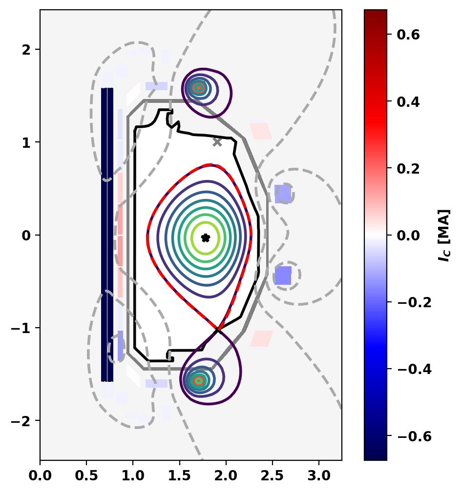
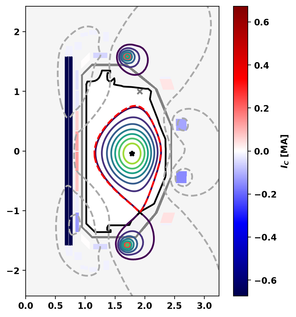
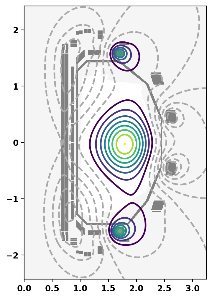
Plot equilibrium

Flux surfaces of the computed equilibrium can be plotted using the plot_psi() method. The additional plotting methods plot_machine() and plot_constraints() are also used to show context and other information. Each method has a large number of optional arguments for formatting and other options.

fig, ax = plt.subplots(1,1)
mygs.plot_machine(fig,ax,coil_colormap='seismic',coil_symmap=True,coil_scale=1.E-6,coil_clabel=r'$I_C$ [MA]')
mygs.plot_psi(fig,ax,vacuum_nlevels=4)
_ = ax.plot(eqdsk['rzout'][:,0], eqdsk['rzout'][:,1],'r--')

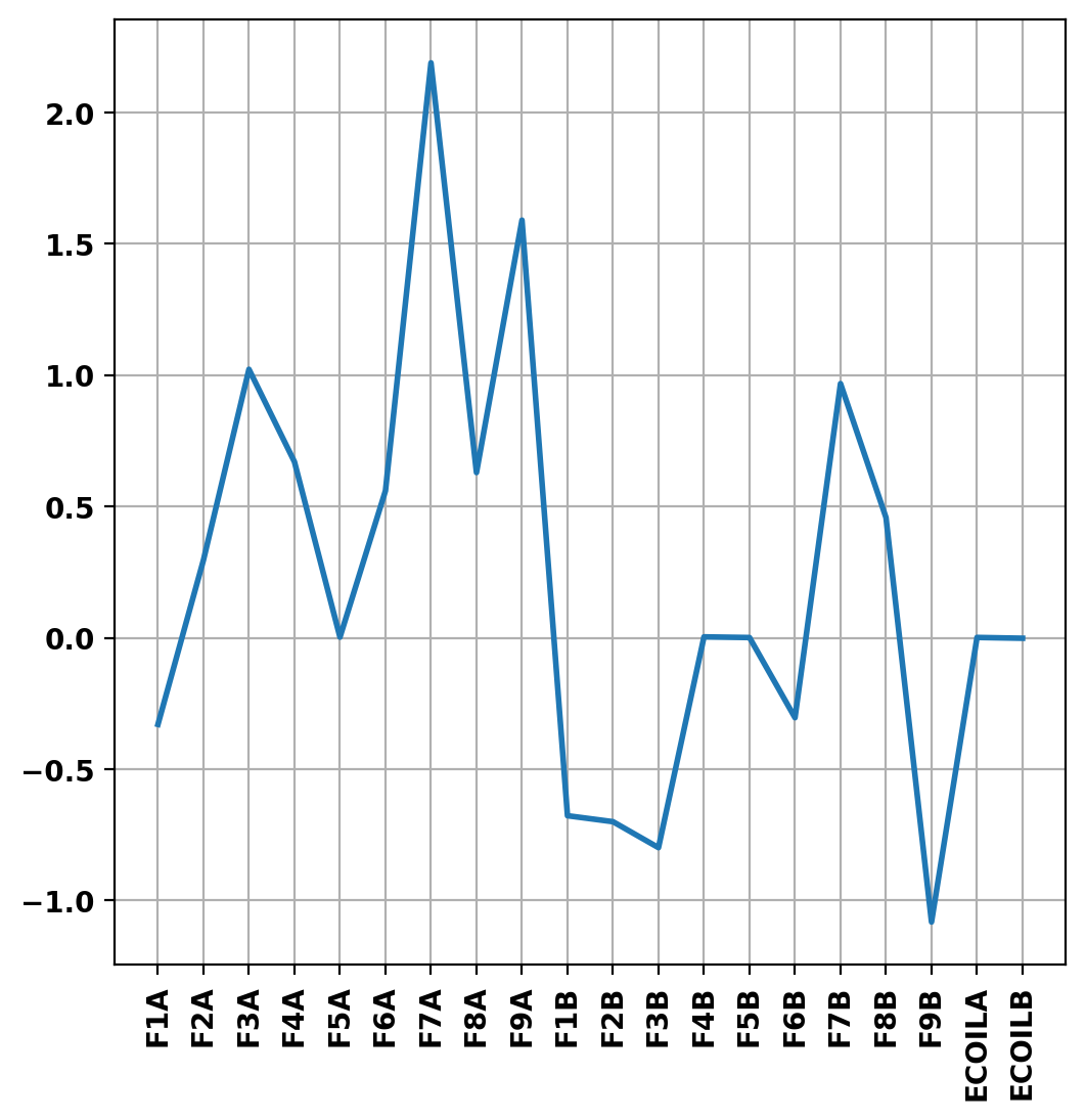
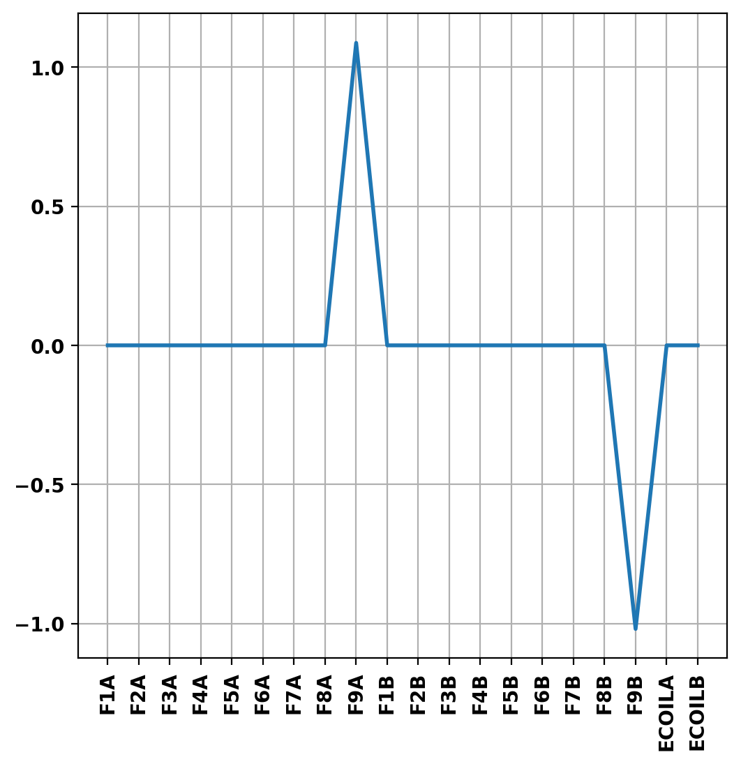
Print equilibrium information and coil currents

Basic parameters can be displayed using the print_info() method. For access to these quantities as variables instead the get_stats() can be used.

The final coil currents can also be retrieved using the get_coil_currents() method. Here, we plot the deviation of the TokaMaker currents from the desired target currents set above.

mygs.print_info()
 
currents, _ = mygs.get_coil_currents()
err = []
keys = []
for key in currents:
    if key.startswith('A') or key.startswith('B'):
        continue
    err.append(100*(target_currents[key]-currents[key])/max(1.E3,abs(target_currents[key])))
    keys.append(key)
    print('  {0:10} {1:10.2F} {2:10.2F} {3:10.2F}'.format(key+":",currents[key]/1.E3,target_currents[key]/1.E3,100*abs((target_currents[key]-currents[key]))/max(1.E3,abs(target_currents[key]))))
plt.plot(range(len(keys)),err)
plt.grid(True)
_ =plt.xticks(range(len(keys)), keys, rotation='vertical')

Equilibrium Statistics:
  Topology                =   Diverted
  Toroidal Current [A]    =    4.9332E+05
  Current Centroid [m]    =    1.758 -0.042
  Magnetic Axis [m]       =    1.780 -0.036
  Elongation              =    1.598 (U:  1.412, L:  1.784)
  Triangularity           =   -0.296 (U: -0.224, L: -0.368)
  Plasma Volume [m^3]     =   14.397
  q_0, q_95               =    0.849  5.386
  Plasma Pressure [Pa]    =   Axis:  6.8216E+03, Peak:  6.8216E+03
  Stored Energy [J]       =    3.9480E+04
  <Beta_pol> [%]          =   23.4009
  <Beta_tor> [%]          =    0.1278
  <Beta_n>   [%]          =    0.2731
  Diamagnetic flux [Wb]   =    6.1406E-03
  Toroidal flux [Wb]      =    2.5085E+00
  l_i                     =    1.6478
  F1A:           116.35     115.97       0.33
  F2A:            59.63      59.81       0.30
  F3A:           -31.07     -30.76       1.02
  F4A:           -40.38     -40.11       0.67
  F5A:             0.72       0.72       0.00
  F6A:          -118.52    -117.86       0.56
  F7A:            33.38      34.13       2.19
  F8A:           -56.96     -56.60       0.63
  F9A:           232.86     236.63       1.59
  F1B:           129.24     128.37       0.68
  F2B:            76.90      76.37       0.70
  F3B:           -22.17     -22.35       0.80
  F4B:          -133.15    -133.14       0.00
  F5B:             0.40       0.40       0.00
  F6B:          -153.10    -153.57       0.30
  F7B:            41.11      41.51       0.97
  F8B:           -51.62     -51.39       0.46
  F9B:           255.11     252.38       1.08
  ECOILA:        -16.03     -16.03       0.00
  ECOILB:        -15.78     -15.78       0.00

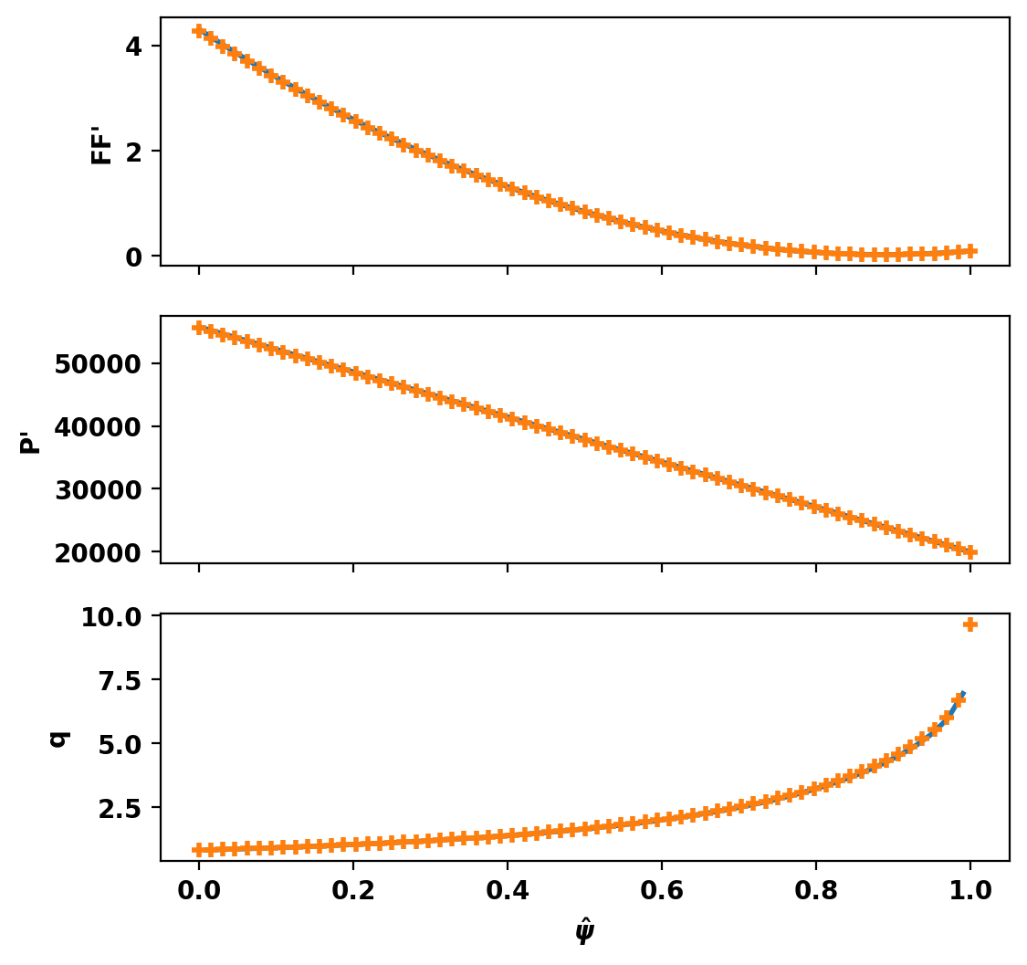
Retrieve profile information

Here, we use get_profiles() and get_q()to obtain the profiles of our equilibrium and compare them to the profiles of the target gEQDSK.

psi,f,fp,p,pp = mygs.get_profiles()
psi_q,qvals,ravgs,dl,rbounds,zbounds = mygs.get_q(psi_pad=0.01)
fig, ax = plt.subplots(3,1,sharex=True)
psi_eqdsk = np.linspace(0.0,1.0,eqdsk['nr'])
psi_sample = np.linspace(0.0,1.0,10)
# Plot F*F'
ax[0].plot(psi,f*fp)
ax[0].plot(psi_eqdsk,-eqdsk['ffprim'],'+')
ax[0].set_ylabel("FF'")
# Plot P'
ax[1].plot(psi,pp)
ax[1].plot(psi_eqdsk,-eqdsk['pprime'],'+')
ax[1].set_ylabel("P'")
# Plot q
ax[2].plot(psi_q,qvals)
ax[2].plot(psi_eqdsk,eqdsk['qpsi'],'+')
ax[2].set_ylabel("q")
_ = ax[-1].set_xlabel(r"$\hat{\psi}$")

Compute Forward (Direct) Equilibrium

Instead of using a coil regularization matrix to reach the desired coil currents, the target coil current values can also be set directly using the set_coil_currents() method. For a direct solve such as this, the isoflux and saddle constraints previously imposed should be removed. We also set new global targets to constrain the axis pressure and vertical position.

mygs.set_isoflux(None)
mygs.set_coil_currents(target_currents)
mygs.set_targets(Ip=eqdsk['ip'],pax=eqdsk['pres'][0],V0=eqdsk['zaxis'])

Compute equilibrium

mygs.solve()

Starting non-linear GS solver
     1 -2.0137E+00 -1.2595E-06  1.2956E-04  1.7801E+00 -3.5537E-02 -4.7738E+03
     2 -2.0243E+00 -1.2630E-06  4.5152E-04  1.7804E+00 -3.6420E-02 -1.2555E+04
     3 -2.0736E+00 -1.2760E-06  1.5659E-04  1.7810E+00 -3.7484E-02 -8.6298E+03
     4 -2.0814E+00 -1.2580E-06  1.1574E-04  1.7815E+00 -3.8576E-02 -7.7634E+03
     5 -2.0843E+00 -1.2534E-06  1.0200E-04  1.7821E+00 -3.9676E-02 -7.4551E+03
     6 -2.0879E+00 -1.2528E-06  1.0519E-04  1.7825E+00 -4.0779E-02 -7.1880E+03
     7 -2.0916E+00 -1.2524E-06  1.5420E-04  1.7830E+00 -4.2057E-02 -8.4448E+03
     8 -2.1038E+00 -1.2549E-06  6.0032E-04  1.7835E+00 -4.2138E-02  4.2058E+03
     9 -2.0424E+00 -1.2290E-06  2.0731E-04  1.7837E+00 -4.2154E-02 -3.0018E+03
    10 -2.0479E+00 -1.2543E-06  6.3538E-05  1.7839E+00 -4.2157E-02 -2.7746E+03
    11 -2.0500E+00 -1.2556E-06  2.7999E-05  1.7841E+00 -4.2158E-02 -2.5962E+03
    12 -2.0498E+00 -1.2546E-06  2.2575E-05  1.7843E+00 -4.2158E-02 -2.5999E+03
    13 -2.0500E+00 -1.2544E-06  2.1837E-05  1.7845E+00 -4.2158E-02 -2.5950E+03
    14 -2.0502E+00 -1.2543E-06  2.8517E-05  1.7847E+00 -4.2158E-02 -2.6250E+03
    15 -2.0506E+00 -1.2542E-06  2.3518E-05  1.7849E+00 -4.2158E-02 -2.6149E+03
    16 -2.0510E+00 -1.2541E-06  2.6083E-05  1.7850E+00 -4.2159E-02 -2.5706E+03
    17 -2.0515E+00 -1.2539E-06  2.1792E-05  1.7852E+00 -4.2159E-02 -2.5705E+03
    18 -2.0517E+00 -1.2537E-06  1.4458E-05  1.7853E+00 -4.2159E-02 -2.5662E+03
    19 -2.0518E+00 -1.2535E-06  1.3539E-05  1.7855E+00 -4.2159E-02 -2.5551E+03
    20 -2.0519E+00 -1.2535E-06  1.4548E-05  1.7856E+00 -4.2159E-02 -2.5670E+03
    21 -2.0522E+00 -1.2534E-06  1.6743E-05  1.7857E+00 -4.2159E-02 -2.5536E+03
    22 -2.0523E+00 -1.2533E-06  1.6311E-05  1.7858E+00 -4.2159E-02 -2.5612E+03
    23 -2.0525E+00 -1.2532E-06  9.7082E-06  1.7859E+00 -4.2159E-02 -2.5647E+03
    24 -2.0527E+00 -1.2532E-06  1.1528E-05  1.7860E+00 -4.2159E-02 -2.5744E+03
    25 -2.0528E+00 -1.2531E-06  1.6957E-05  1.7861E+00 -4.2159E-02 -2.5705E+03
    26 -2.0531E+00 -1.2531E-06  1.6802E-05  1.7861E+00 -4.2159E-02 -2.5629E+03
    27 -2.0533E+00 -1.2530E-06  1.2792E-05  1.7862E+00 -4.2159E-02 -2.5687E+03
    28 -2.0534E+00 -1.2530E-06  1.7785E-05  1.7863E+00 -4.2159E-02 -2.5593E+03
    29 -2.0536E+00 -1.2529E-06  1.6300E-05  1.7864E+00 -4.2159E-02 -2.5410E+03
    30 -2.0537E+00 -1.2529E-06  1.5765E-05  1.7864E+00 -4.2159E-02 -2.5319E+03
    31 -2.0539E+00 -1.2528E-06  9.3532E-06  1.7865E+00 -4.2159E-02 -2.5242E+03
    32 -2.0539E+00 -1.2527E-06  9.6777E-06  1.7866E+00 -4.2159E-02 -2.5233E+03
    33 -2.0541E+00 -1.2528E-06  1.0426E-05  1.7866E+00 -4.2159E-02 -2.5116E+03
    34 -2.0543E+00 -1.2527E-06  1.0136E-05  1.7867E+00 -4.2159E-02 -2.5265E+03
    35 -2.0545E+00 -1.2527E-06  4.3841E-06  1.7867E+00 -4.2159E-02 -2.5351E+03
    36 -2.0546E+00 -1.2527E-06  1.0404E-05  1.7867E+00 -4.2159E-02 -2.5347E+03
    37 -2.0547E+00 -1.2526E-06  9.2006E-06  1.7868E+00 -4.2159E-02 -2.5311E+03
    38 -2.0547E+00 -1.2526E-06  3.5156E-06  1.7868E+00 -4.2159E-02 -2.5255E+03
    39 -2.0548E+00 -1.2526E-06  9.2578E-06  1.7869E+00 -4.2159E-02 -2.5262E+03
    40 -2.0548E+00 -1.2525E-06  3.2335E-06  1.7869E+00 -4.2159E-02 -2.5102E+03
    41 -2.0548E+00 -1.2525E-06  9.0317E-06  1.7869E+00 -4.2159E-02 -2.5111E+03
    42 -2.0548E+00 -1.2525E-06  3.0114E-06  1.7869E+00 -4.2159E-02 -2.5198E+03
    43 -2.0548E+00 -1.2525E-06  5.6320E-06  1.7870E+00 -4.2159E-02 -2.5194E+03
    44 -2.0549E+00 -1.2525E-06  5.3106E-06  1.7870E+00 -4.2159E-02 -2.5216E+03
    45 -2.0549E+00 -1.2525E-06  1.0432E-05  1.7870E+00 -4.2159E-02 -2.5184E+03
    46 -2.0549E+00 -1.2525E-06  6.1186E-06  1.7870E+00 -4.2159E-02 -2.5174E+03
    47 -2.0549E+00 -1.2525E-06  1.4365E-05  1.7871E+00 -4.2159E-02 -2.5191E+03
    48 -2.0551E+00 -1.2525E-06  1.4332E-05  1.7871E+00 -4.2159E-02 -2.5326E+03
    49 -2.0553E+00 -1.2525E-06  5.3658E-06  1.7871E+00 -4.2159E-02 -2.5386E+03
    50 -2.0555E+00 -1.2524E-06  1.4133E-05  1.7871E+00 -4.2159E-02 -2.5419E+03
    51 -2.0557E+00 -1.2524E-06  3.7620E-06  1.7872E+00 -4.2159E-02 -2.5605E+03
    52 -2.0558E+00 -1.2523E-06  1.5590E-05  1.7872E+00 -4.2159E-02 -2.5609E+03
    53 -2.0559E+00 -1.2523E-06  3.9554E-06  1.7872E+00 -4.2159E-02 -2.5514E+03
    54 -2.0560E+00 -1.2522E-06  2.4260E-06  1.7872E+00 -4.2159E-02 -2.5527E+03
    55 -2.0560E+00 -1.2522E-06  5.0169E-06  1.7873E+00 -4.2159E-02 -2.5531E+03
    56 -2.0560E+00 -1.2522E-06  2.1940E-06  1.7873E+00 -4.2159E-02 -2.5605E+03
    57 -2.0561E+00 -1.2522E-06  1.7743E-06  1.7873E+00 -4.2159E-02 -2.5605E+03
    58 -2.0561E+00 -1.2522E-06  1.5630E-06  1.7873E+00 -4.2159E-02 -2.5606E+03
    59 -2.0562E+00 -1.2522E-06  1.3824E-06  1.7873E+00 -4.2159E-02 -2.5607E+03
    60 -2.0562E+00 -1.2521E-06  1.2228E-06  1.7874E+00 -4.2159E-02 -2.5608E+03
    61 -2.0562E+00 -1.2521E-06  6.4068E-06  1.7874E+00 -4.2159E-02 -2.5609E+03
    62 -2.0562E+00 -1.2521E-06  1.7075E-06  1.7874E+00 -4.2159E-02 -2.5701E+03
    63 -2.0563E+00 -1.2521E-06  1.0225E-06  1.7874E+00 -4.2159E-02 -2.5697E+03
    64 -2.0563E+00 -1.2521E-06  4.7539E-06  1.7874E+00 -4.2159E-02 -2.5697E+03
    65 -2.0563E+00 -1.2521E-06  4.5549E-06  1.7874E+00 -4.2159E-02 -2.5641E+03
    66 -2.0563E+00 -1.2521E-06  1.2642E-06  1.7874E+00 -4.2159E-02 -2.5724E+03
    67 -2.0563E+00 -1.2521E-06  7.8325E-07  1.7874E+00 -4.2159E-02 -2.5720E+03
 Timing:  0.74570699996547773     
   Source:    0.30776199983665720     
   Solve:     0.33583900035591796     
   Boundary:   2.4080999719444662E-002
   Other:      7.8025000053457916E-002

Print equilibrium information and coil currents

Here we plot the output of the direct solve, which shows close agreement with the desired plasma boundary. We also print the equilibrium information and plot the error in the coil currents. Because the coil currents were set explicitely, there is no deviation between the target and actual currents, except in the vertical stability coil pair.

fig, ax = plt.subplots(1,1)
mygs.plot_machine(fig,ax,coil_colormap='seismic',coil_symmap=True,coil_scale=1.E-6,coil_clabel=r'$I_C$ [MA]')
mygs.plot_psi(fig,ax,vacuum_nlevels=4)
ax.plot(eqdsk['rzout'][:,0], eqdsk['rzout'][:,1],'r--')

[<matplotlib.lines.Line2D at 0x134bd8b90>]

mygs.print_info()
 
currents, _ = mygs.get_coil_currents()
err = []
keys = []
for key in currents:
    if key.startswith('A') or key.startswith('B'):
        continue
    err.append(100*(target_currents[key]-currents[key])/max(1.E3,abs(target_currents[key])))
    keys.append(key)
    print('  {0:10} {1:10.2F} {2:10.2F} {3:10.2F}'.format(key+":",currents[key]/1.E3,target_currents[key]/1.E3,100*abs((target_currents[key]-currents[key]))/max(1.E3,abs(target_currents[key]))))
plt.plot(range(len(keys)),err)
plt.grid(True)
_ =plt.xticks(range(len(keys)), keys, rotation='vertical')

Equilibrium Statistics:
  Topology                =   Limited
  Toroidal Current [A]    =    4.9332E+05
  Current Centroid [m]    =    1.766 -0.048
  Magnetic Axis [m]       =    1.787 -0.042
  Elongation              =    1.603 (U:  1.408, L:  1.798)
  Triangularity           =   -0.286 (U: -0.210, L: -0.362)
  Plasma Volume [m^3]     =   14.283
  q_0, q_95               =    0.829  5.251
  Plasma Pressure [Pa]    =   Axis:  6.8216E+03, Peak:  6.8216E+03
  Stored Energy [J]       =    3.9108E+04
  <Beta_pol> [%]          =   22.9405
  <Beta_tor> [%]          =    0.1291
  <Beta_n>   [%]          =    0.2718
  Diamagnetic flux [Wb]   =    6.1909E-03
  Toroidal flux [Wb]      =    2.4632E+00
  l_i                     =    1.6428
  F1A:           115.97     115.97       0.00
  F2A:            59.81      59.81       0.00
  F3A:           -30.76     -30.76       0.00
  F4A:           -40.11     -40.11       0.00
  F5A:             0.72       0.72       0.00
  F6A:          -117.86    -117.86       0.00
  F7A:            34.13      34.13       0.00
  F8A:           -56.60     -56.60       0.00
  F9A:           234.05     236.63       1.09
  F1B:           128.37     128.37       0.00
  F2B:            76.37      76.37       0.00
  F3B:           -22.35     -22.35       0.00
  F4B:          -133.14    -133.14       0.00
  F5B:             0.40       0.40       0.00
  F6B:          -153.57    -153.57       0.00
  F7B:            41.51      41.51       0.00
  F8B:           -51.39     -51.39       0.00
  F9B:           254.95     252.38       1.02
  ECOILA:        -16.03     -16.03       0.00
  ECOILB:        -15.78     -15.78       0.00

Save equilibrium as a gEQDSK file

We save our TokaMaker equilibrium as a gEQDSK file using the save_eqdsk() method. We modify the resolution of the equilibrium file by increasing the nr and nz parameters and decreasing the padding on the last closed flux surface (lcfs_pad).

mygs.save_eqdsk('g192185_tokamaker', nr = 200, nz = 200, lcfs_pad = 0.001)

Saving gEQDSK: g192185_tokamaker

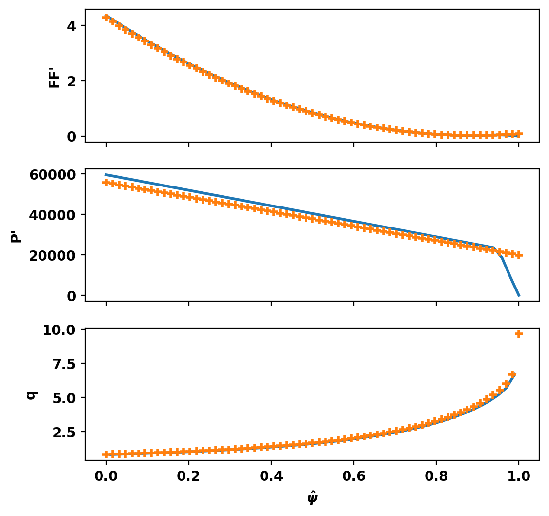
Update equilibrium for linear stability

As is often the case with experimental equilibrium reconstructions, the profiles provided in the gEQDSK file have unrealistically high edge current ( \( F*F' \) and \( P' \) at the LCFS). To improve the behavior of the equilibrium during stability and time-dependent solves we apply a simple linear ramp to drop both \( F*F' \) and \( P' \) to zero at \( \hat{\psi} = 1 \).

Warning: Even when matching global quantities, this change will modify the stability and time-dependent properties of the equilibrium. Therefore care should always be taken with such a modification to avoid trading on unphysical profile for another.

Additionally, we change the form of our targets to use Ip_ratio instead of pax. This form allows us to later perform a VDE simulation with constant \( I_p \) and roughly constant \( \beta_p \).

We then recompute the equilibrium to prepare for time-dependent analysis.

# Modify profiles to remove edge current
edge_ramp = (1.0-ffp_prof[:,0])/(0.05)
edge_ramp[edge_ramp > 1.0] = 1.0
mygs.set_profiles(ffp_prof={'type': 'linterp', 'y': edge_ramp*ffp_prof[:,1], 'x': ffp_prof[:,0]},
                  pp_prof={'type': 'linterp', 'y': edge_ramp*pp_prof[:,1], 'x': pp_prof[:,0]})
# Update global targets
mygs.set_targets(Ip=eqdsk['ip'],Ip_ratio=5.6,V0=eqdsk['zaxis'])
# Recompute equilibrim
mygs.solve()

Starting non-linear GS solver
     1 -2.0641E+00 -1.3630E-06  1.6090E-04  1.7878E+00 -4.2159E-02 -4.0962E+03
     2 -2.0459E+00 -1.3506E-06  6.6897E-05  1.7881E+00 -4.2159E-02 -4.3025E+03
     3 -2.0373E+00 -1.3471E-06  3.5098E-05  1.7883E+00 -4.2159E-02 -4.3272E+03
     4 -2.0332E+00 -1.3458E-06  2.1819E-05  1.7885E+00 -4.2159E-02 -4.3284E+03
     5 -2.0314E+00 -1.3453E-06  1.6475E-05  1.7887E+00 -4.2159E-02 -4.3270E+03
     6 -2.0306E+00 -1.3450E-06  1.4258E-05  1.7889E+00 -4.2159E-02 -4.3261E+03
     7 -2.0304E+00 -1.3449E-06  1.3049E-05  1.7890E+00 -4.2159E-02 -4.3255E+03
     8 -2.0304E+00 -1.3448E-06  1.2141E-05  1.7892E+00 -4.2159E-02 -4.3253E+03
     9 -2.0305E+00 -1.3447E-06  1.1339E-05  1.7893E+00 -4.2159E-02 -4.3254E+03
    10 -2.0307E+00 -1.3446E-06  1.0597E-05  1.7894E+00 -4.2159E-02 -4.3255E+03
    11 -2.0309E+00 -1.3446E-06  9.9013E-06  1.7896E+00 -4.2159E-02 -4.3256E+03
    12 -2.0311E+00 -1.3445E-06  9.2487E-06  1.7897E+00 -4.2159E-02 -4.3257E+03
    13 -2.0313E+00 -1.3445E-06  8.6376E-06  1.7898E+00 -4.2159E-02 -4.3257E+03
    14 -2.0314E+00 -1.3445E-06  8.0659E-06  1.7899E+00 -4.2159E-02 -4.3258E+03
    15 -2.0316E+00 -1.3444E-06  7.5326E-06  1.7900E+00 -4.2159E-02 -4.3260E+03
    16 -2.0318E+00 -1.3444E-06  7.0351E-06  1.7900E+00 -4.2159E-02 -4.3262E+03
    17 -2.0319E+00 -1.3444E-06  6.5703E-06  1.7901E+00 -4.2159E-02 -4.3263E+03
    18 -2.0320E+00 -1.3444E-06  6.1358E-06  1.7902E+00 -4.2159E-02 -4.3265E+03
    19 -2.0322E+00 -1.3443E-06  5.7299E-06  1.7903E+00 -4.2159E-02 -4.3267E+03
    20 -2.0323E+00 -1.3443E-06  5.3509E-06  1.7903E+00 -4.2159E-02 -4.3268E+03
    21 -2.0324E+00 -1.3443E-06  4.9972E-06  1.7904E+00 -4.2159E-02 -4.3270E+03
    22 -2.0325E+00 -1.3443E-06  4.6666E-06  1.7904E+00 -4.2159E-02 -4.3272E+03
    23 -2.0326E+00 -1.3442E-06  4.3580E-06  1.7905E+00 -4.2159E-02 -4.3273E+03
    24 -2.0327E+00 -1.3442E-06  4.0698E-06  1.7905E+00 -4.2159E-02 -4.3274E+03
    25 -2.0328E+00 -1.3442E-06  3.8007E-06  1.7906E+00 -4.2159E-02 -4.3275E+03
    26 -2.0329E+00 -1.3442E-06  3.5495E-06  1.7906E+00 -4.2159E-02 -4.3276E+03
    27 -2.0329E+00 -1.3442E-06  3.3146E-06  1.7907E+00 -4.2159E-02 -4.3278E+03
    28 -2.0330E+00 -1.3442E-06  3.0949E-06  1.7907E+00 -4.2159E-02 -4.3279E+03
    29 -2.0331E+00 -1.3442E-06  2.8897E-06  1.7907E+00 -4.2159E-02 -4.3280E+03
    30 -2.0331E+00 -1.3441E-06  2.6981E-06  1.7908E+00 -4.2159E-02 -4.3281E+03
    31 -2.0332E+00 -1.3441E-06  2.5190E-06  1.7908E+00 -4.2159E-02 -4.3282E+03
    32 -2.0332E+00 -1.3441E-06  2.3520E-06  1.7908E+00 -4.2159E-02 -4.3283E+03
    33 -2.0333E+00 -1.3441E-06  2.1961E-06  1.7909E+00 -4.2159E-02 -4.3284E+03
    34 -2.0333E+00 -1.3441E-06  2.0508E-06  1.7909E+00 -4.2159E-02 -4.3285E+03
    35 -2.0334E+00 -1.3441E-06  1.9149E-06  1.7909E+00 -4.2159E-02 -4.3286E+03
    36 -2.0334E+00 -1.3441E-06  1.7881E-06  1.7909E+00 -4.2159E-02 -4.3287E+03
    37 -2.0335E+00 -1.3441E-06  1.6695E-06  1.7910E+00 -4.2159E-02 -4.3288E+03
    38 -2.0335E+00 -1.3441E-06  1.5587E-06  1.7910E+00 -4.2159E-02 -4.3288E+03
    39 -2.0335E+00 -1.3441E-06  1.4553E-06  1.7910E+00 -4.2159E-02 -4.3289E+03
    40 -2.0335E+00 -1.3441E-06  1.3586E-06  1.7910E+00 -4.2159E-02 -4.3290E+03
    41 -2.0336E+00 -1.3441E-06  1.2683E-06  1.7910E+00 -4.2159E-02 -4.3290E+03
    42 -2.0336E+00 -1.3441E-06  1.1840E-06  1.7910E+00 -4.2159E-02 -4.3291E+03
    43 -2.0336E+00 -1.3441E-06  1.1053E-06  1.7910E+00 -4.2159E-02 -4.3291E+03
    44 -2.0337E+00 -1.3441E-06  1.0319E-06  1.7911E+00 -4.2159E-02 -4.3292E+03
    45 -2.0337E+00 -1.3441E-06  9.6340E-07  1.7911E+00 -4.2159E-02 -4.3292E+03
 Timing:  0.50464100000681356     
   Source:    0.20982700004242361     
   Solve:     0.22672400006558746     
   Boundary:   1.5833999961614609E-002
   Other:      5.2255999937187880E-002

Plot profile information

Again we use get_profiles() to compare the updated profiles with the initial gEQDSK profiles and visualize the local modifications introduced at the edge.

psi,f,fp,p,pp = mygs.get_profiles()
psi_q,qvals,ravgs,dl,rbounds,zbounds = mygs.get_q(psi_pad=0.01)
fig, ax = plt.subplots(3,1,sharex=True)
psi_eqdsk = np.linspace(0.0,1.0,eqdsk['nr'])
psi_sample = np.linspace(0.0,1.0,10)
# Plot F*F'
ax[0].plot(psi,f*fp)
ax[0].plot(psi_eqdsk,-eqdsk['ffprim'],'+')
ax[0].set_ylabel("FF'")
# Plot P'
ax[1].plot(psi,pp)
ax[1].plot(psi_eqdsk,-eqdsk['pprime'],'+')
ax[1].set_ylabel("P'")
# Plot q
ax[2].plot(psi_q,qvals)
ax[2].plot(psi_eqdsk,eqdsk['qpsi'],'+')
ax[2].set_ylabel("q")
_ = ax[-1].set_xlabel(r"$\hat{\psi}$")

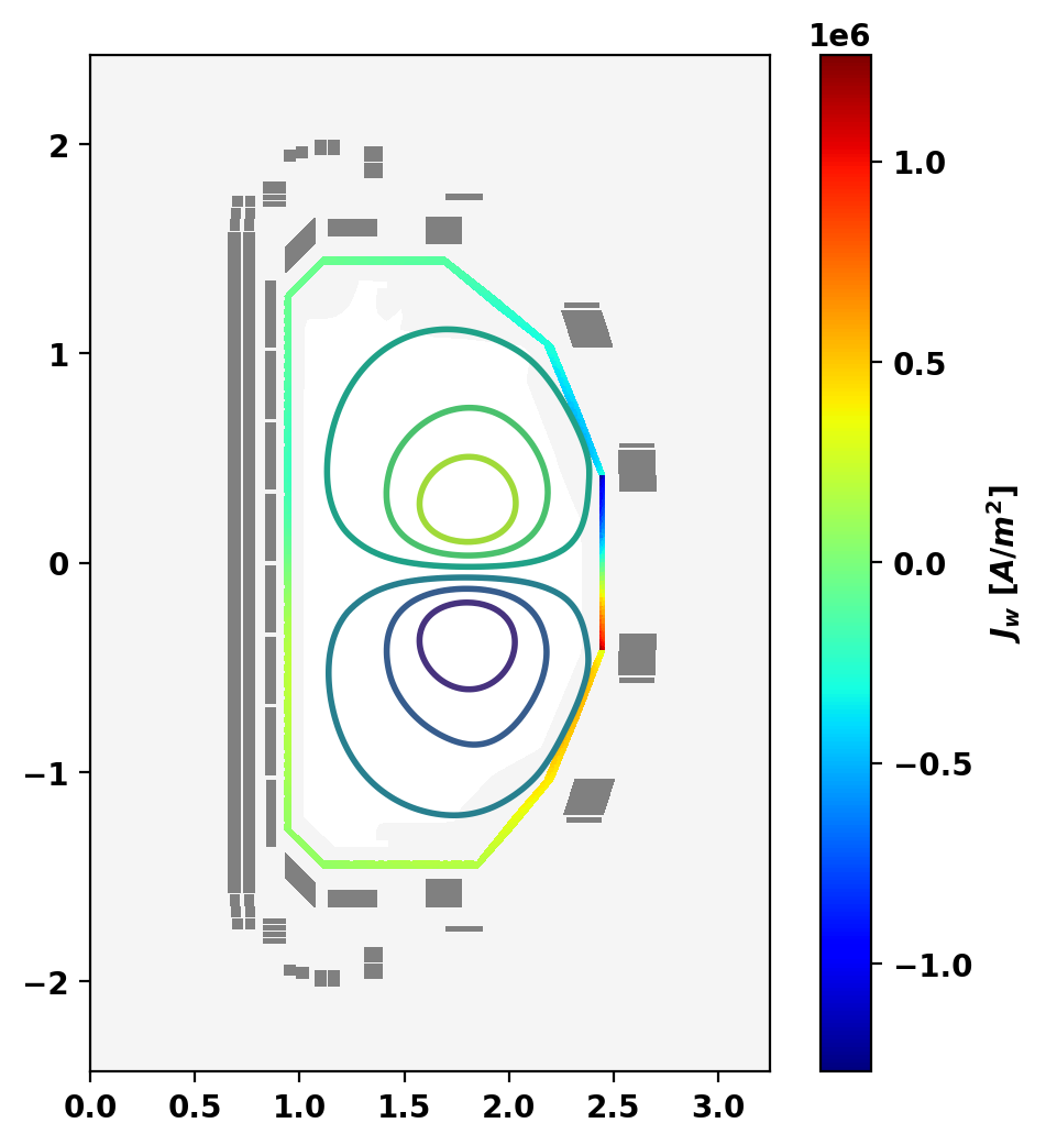
Linear Stability Analysis

We can compute the most unstable eigenmodes of the linearized system along with their eigenvalues, or growth rates, using the eig_td() method. In this case, the most unstable mode corresponds to vertical instability, and has a growth rate of ~807 s^-1.

We also plot the vertically unstable mode and the eddy currents in conducting structures using the plot_eddy() method.

eig_vals, eig_vecs = mygs.eig_td(-5.E3,10,False) 
fig, ax = plt.subplots()
mygs.plot_machine(fig,ax,limiter_color=None)
mygs.plot_psi(fig,ax,eig_vecs[0,:],normalized=False,xpoint_color=None,opoint_color=None)
mygs.plot_eddy(fig,ax,dpsi_dt=eig_vecs[0,:]*abs(eig_vals[0,0]))
print('Growth rate = {0:.4E} [s^-1]'.format(-eig_vals[0,0]))
print('Growth time = {0:.4E} [s]'.format(-1.0/eig_vals[0,0]))

Growth rate = 9.4598E+02 [s^-1]
Growth time = 1.0571E-03 [s]

Time-dependent VDE simulation

A VDE can be initiated by extracting the original equilibrium \(\psi\) using get_psi() and adding a perturbation corresponding to the vertically unstable eigenmode. Then, set_psi() can be used to set this modified equilibrium as the initial condition for the time dependent simulation. The modified equilibrium is visualized below.

psi0 = mygs.get_psi(normalized = False)
max_loc = abs(eig_vecs[0,:]).argmax()
psi_ic = psi0-eig_vecs[0,:]*(mygs.psi_bounds[1]-mygs.psi_bounds[0])/eig_vecs[0,max_loc]/50.0
 
fig, ax = plt.subplots(1,1)
mygs.plot_machine(fig,ax,limiter_color=None)
mygs.plot_psi(fig,ax,(psi_ic-mygs.psi_bounds[1])/(mygs.psi_bounds[0]-mygs.psi_bounds[1]),xpoint_color=None,opoint_color=None)
mygs.set_psi(psi_ic)

Setup simulation

In order to run the time-dependent simulation, the isoflux constraints are removed and the setup_td() method is run to set the initial timestep and tolerances for the solver. A timestep is chosen that aligns with the predicted growth time of the unstable mode.

mygs.settings.pm=False
mygs.update_settings()
mygs.set_isoflux(None)
mygs.set_targets(Ip=eqdsk['ip'],Ip_ratio=5.6)
mygs.setup_td(1.E-03,1.E-13,1.E-11,pre_plasma=False)

Perform time-dependent simulation

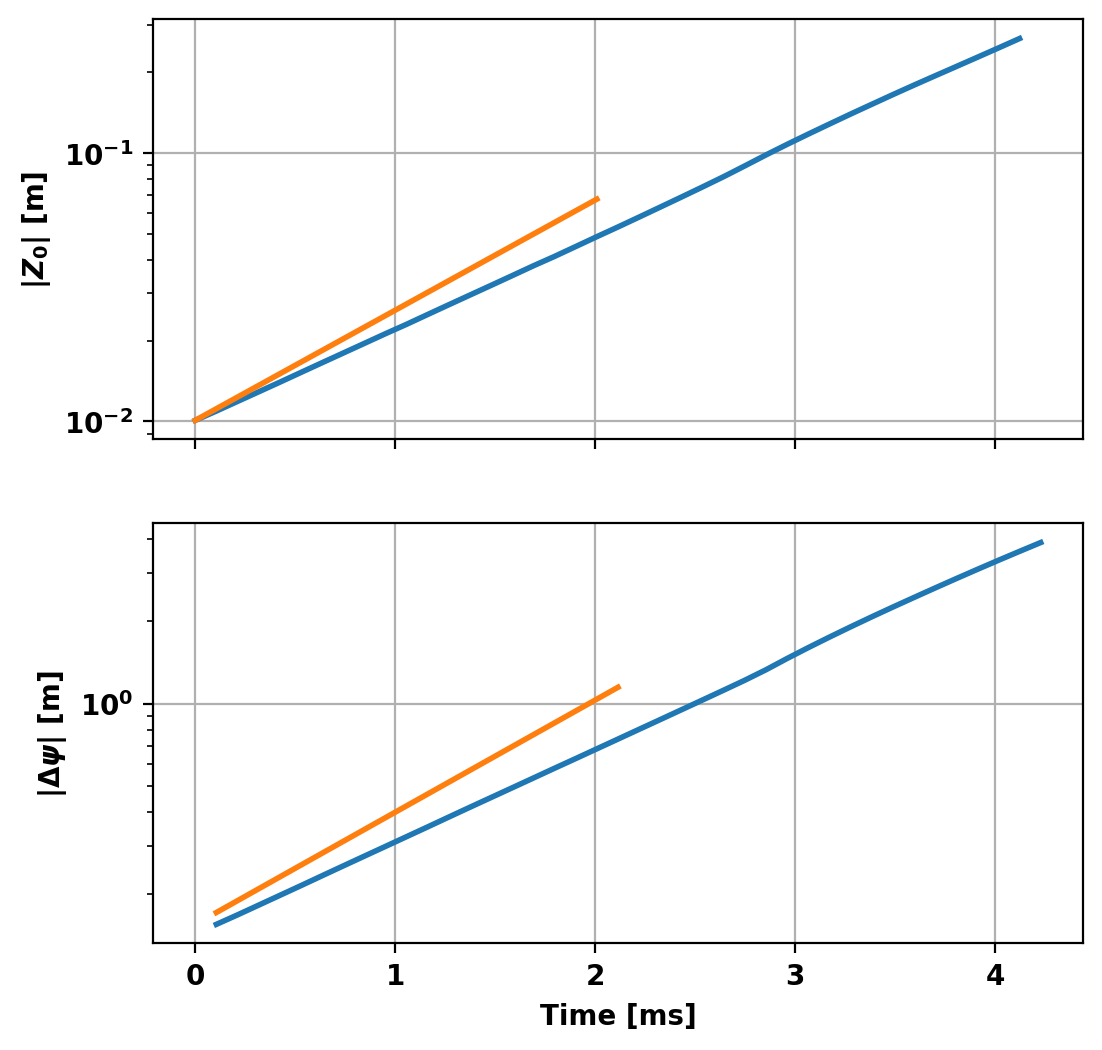
To run the simulation, step_td() is run for the desired number of timesteps. At each timestep, we save \(\psi\) as well as the vertical position of the magnetic axis and the amplitude of the vertically unstable eigenmode.

import time
sim_time = 0.0
dt = 1.E-1/-eig_vals[0,0]
nplot = 1
nstatus = 2
results = [mygs.get_psi()]
results_raw = [mygs.get_psi(False)]
z0 = [[sim_time,mygs.o_point[1]],]
eig_comp = [[sim_time,np.dot(eig_vecs[0,:],mygs.get_psi(normalized=False)-psi0)],]
t00 = time.perf_counter()
 
for i in range(40):
    t0 = time.perf_counter()
    sim_time, _, nl_its, lin_its, nretry = mygs.step_td(sim_time,dt)
    t1 = time.perf_counter()
    if i % nstatus == 0:
        print('{0:.5E} {1:.5E} {2:4d} {3:4d} {5:8.3f} {4:4d}'.format(sim_time,dt,nl_its,lin_its,nretry,t1-t0))
    z0.append([sim_time,mygs.o_point[1]])
    eig_comp.append([sim_time,np.dot(eig_vecs[0,:],mygs.get_psi(normalized=False)-psi0)])
    if i % nplot == 0:
        results.append(mygs.get_psi())
        results_raw.append(mygs.get_psi(False))
t1 = time.perf_counter()
print('Total time = {0:8.3f}'.format(t1-t00))

1.05711E-04 1.05711E-04    2   16    0.320    0
3.17132E-04 1.05711E-04    2   15    0.247    0
5.28554E-04 1.05711E-04    2   16    0.172    0
7.39976E-04 1.05711E-04    2   16    0.169    0
9.51397E-04 1.05711E-04    2   16    0.168    0
1.16282E-03 1.05711E-04    2   17    0.178    0
1.37424E-03 1.05711E-04    2   18    0.186    0
1.58566E-03 1.05711E-04    2   18    0.195    0
1.79708E-03 1.05711E-04    2   18    0.188    0
2.00851E-03 1.05711E-04    2   18    0.188    0
2.21993E-03 1.05711E-04    2   18    0.188    0
2.43135E-03 1.05711E-04    2   18    0.190    0
2.64277E-03 1.05711E-04    2   18    0.187    0
2.85419E-03 1.05711E-04    3   25    0.260    0
3.06561E-03 1.05711E-04    2   19    0.196    0
3.27704E-03 1.05711E-04    2   19    0.195    0
3.48846E-03 1.05711E-04    2   19    0.194    0
3.69988E-03 1.05711E-04    2   19    0.199    0
3.91130E-03 1.05711E-04    2   19    0.193    0
4.12272E-03 1.05711E-04    3   27    0.268    0
Total time =    8.046

Plot evolution of flux surfaces

We plot the last closed flux surface at each timestep to visualize the plasma evolution.

import matplotlib as mpl
fig, ax = plt.subplots(1,2,constrained_layout=True,figsize=(8,5))
mygs.plot_machine(fig,ax[0])
colors = plt.cm.jet(np.linspace(0,1,len(results)))
for i, result in enumerate(results):
    mygs.plot_psi(fig,ax[0],psi=result,plasma_nlevels=1,plasma_color=[colors[i]], vacuum_nlevels = 0,xpoint_color=None,opoint_color=None)
norm = mpl.colors.Normalize(vmin=0.0, vmax=sim_time*1.E3)
mygs.plot_machine(fig,ax[1])
colors = plt.cm.jet(np.linspace(0,1,len(results)))
for i, result in enumerate(results):
    mygs.plot_psi(fig,ax[1],psi=result,plasma_nlevels=1,plasma_color=[colors[i]], vacuum_nlevels = 0,xpoint_color=None,opoint_color=None)
ax[1].plot(mygs.lim_point[0],mygs.lim_point[1],'ro')
ax[1].triplot(mesh_pts[:,0],mesh_pts[:,1],mesh_lc[mesh_reg==3,:],lw=0.5,label=key)
norm = mpl.colors.Normalize(vmin=0.0, vmax=sim_time*1.E3)
_ = fig.colorbar(mpl.cm.ScalarMappable(norm=norm, cmap=plt.cm.jet),ax=ax[1],label='Time [ms]')
ax[1].set_ylim(-1.3,-0.8)
_ =ax[1].set_xlim(1.6,2.1)

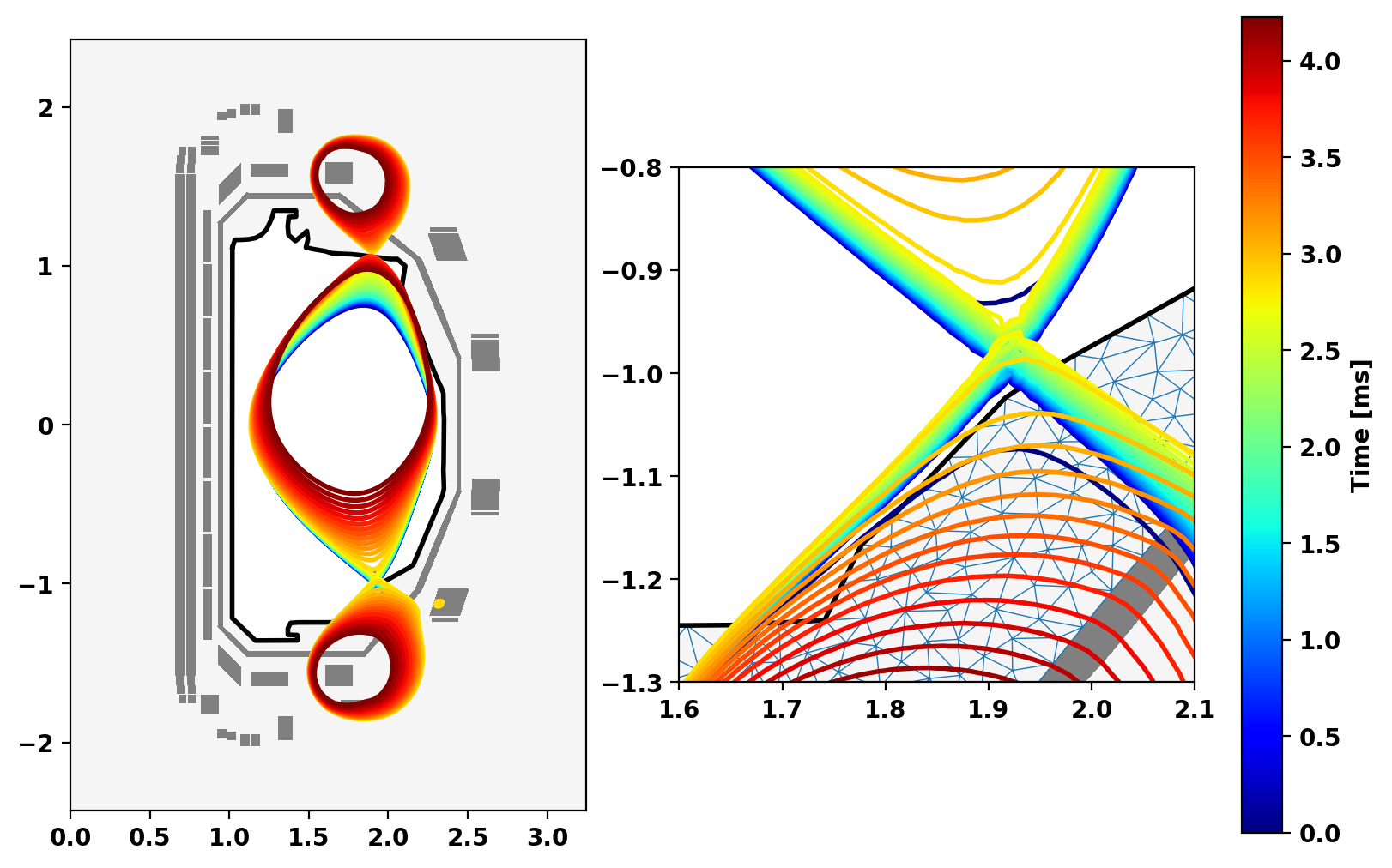
Plot time-evolution of equilibrium

Here we plot the evolution of the vertical position of the plasma and the amplitude of the computed eigenvector from above in the solution (as compared to the initial state). Both of these values should grow linearly at the predicted growth rate (shown in orange).

fig, ax = plt.subplots(2,1,sharex=True)
z_hist = np.asarray(z0); z_hist = z_hist[1:,:] - [z_hist[1,0], z_hist[0,1]]
ax[0].semilogy(z_hist[:,0]*1.E3,abs(z_hist[:,1]))
ax[0].semilogy(z_hist[:20,0]*1.E3,abs(z_hist[0,1])*np.exp(-z_hist[:20,0]*eig_vals[0,0]))
ax[0].set_ylabel(r'$|Z_0|$ [m]')
ax[0].grid(True)
eig_hist = np.asarray(eig_comp); eig_hist = eig_hist[1:,:]
ax[1].semilogy(eig_hist[:,0]*1.E3,abs(eig_hist[:,1]))
ax[1].semilogy(eig_hist[:20,0]*1.E3,abs(eig_hist[0,1])*np.exp(-eig_hist[:20,0]*eig_vals[0,0]))
ax[1].set_ylabel(r'$|\Delta \psi|$ [m]')
ax[1].grid(True)
_ = ax[-1].set_xlabel(r'Time [ms]')