In this example we compute the Taylor state in a R=1, L=10 cylinder with Marklin and then demonstrate tracing the magnetic field and the vector potential.

import os
import sys
import time
import numpy as np
from scipy.integrate import odeint
import matplotlib.pyplot as plt
plt.rcParams['figure.figsize']=(6,6)
plt.rcParams['font.weight']='bold'
plt.rcParams['axes.labelweight']='bold'
plt.rcParams['lines.linewidth']=2
plt.rcParams['lines.markeredgewidth']=2
%matplotlib inline
%config InlineBackend.figure_format = "retina"

Load Marklin library

To load the Marklin python module we need to tell python where to the module is located. This can be done either through the PYTHONPATH environment variable or using within a script using sys.path.append() as below, where we look for the environement variable OFT_ROOTPATH to provide the path to where the OpenFUSIONToolkit is installed (/Applications/OFT on macOS).

tokamaker_python_path = os.getenv('OFT_ROOTPATH')
if tokamaker_python_path is not None:
    sys.path.append(os.path.join(tokamaker_python_path,'python'))
from OpenFUSIONToolkit import OFT_env
from OpenFUSIONToolkit.Marklin import Marklin

Compute equilibria

Initialize Marklin object

First we create a Marklin instance to use for equilibrium calculations.

myOFT = OFT_env(nthreads=4)

taylor_solver = Marklin(myOFT)

#----------------------------------------------
Open FUSION Toolkit Initialized
Development branch:   Marklin_vacuum
Revision id:          1de4a06
Parallelization Info:
  # of MPI tasks      =    1
  # of NUMA nodes     =    1
  # of OpenMP threads =    4
Fortran input file    = /var/folders/52/n5qxh27n4w19qxzqygz2btbw0000gn/T/oft_51889/oftpyin
XML input file        = none
Integer Precisions    =    4   8
Float Precisions      =    4   8  16
Complex Precisions    =    4   8
LA backend            = native
#----------------------------------------------

Load mesh

Now we load a mesh of the desired region generated using Cubit using setup_mesh().

taylor_solver.setup_mesh(mesh_file='cyl10_mesh.h5',grid_order=2)

taylor_solver.setup(order=2,minlev=1)

**** Loading OFT mesh
  Mesh File = cyl10_mesh.h5

**** Generating grid level  1
  Generating domain linkage
  Generating boundary domain linkage
  Mesh statistics:
    Volume          =  3.125E+01
    Surface area    =  6.899E+01
    # of points     =    6867
    # of edges      =   43660
    # of faces      =   71594
    # of cells      =   34800
    # of boundary points =    1996
    # of boundary edges  =    5982
    # of boundary faces  =    3988
    # of boundary cells  =    3928
  Resolution statistics:
    hmin =  1.101E-01
    hrms =  2.077E-01
    hmax =  3.575E-01
  Surface grounded at vertex    1482


**** Creating Lagrange FE space
  Order  =    2
  Minlev =    1


**** Creating H(Curl) FE space
  Order  =    2
  Minlev =    1



WARNING: No Lagrange MG smoother settings found:
WARNING:   Using default values, which may result in convergence failure.
WARNING: No H(Curl) MG smoother settings found:
WARNING:   Using default values, which may result in convergence failure.

Compute eigenmodes

We now use compute_eig() to compute the force-free eigenstates of the system \(\textbf{J} = \lambda \textbf{B}\).

taylor_solver.compute_eig(1)

Starting calculation of Taylor states

Starting CG eigensolver 0 1.913621E+04 2.029553E+06 1 6.903028E+01 2.252654E+01 2 3.783637E+01 9.375920E+00 3 2.596353E+01 5.974242E+00 4 2.047505E+01 4.059782E+00 5 1.720316E+01 2.837043E+00 6 1.499618E+01 2.263157E+00 7 1.326034E+01 2.022059E+00 8 1.189920E+01 1.727096E+00 9 1.091428E+01 1.498545E+00 10 1.018982E+01 1.229505E+00 20 6.339615E+00 8.829472E-01 30 4.894643E+00 4.400030E-01 40 4.278360E+00 2.027685E-01 50 4.013336E+00 9.194628E-02 60 3.887575E+00 6.052810E-02 70 3.782666E+00 6.310277E-02 80 3.663833E+00 8.411119E-02 90 3.551018E+00 5.660238E-02 100 3.483311E+00 4.075690E-02 110 3.423870E+00 3.593544E-02 120 3.377094E+00 2.834637E-02 130 3.342751E+00 2.001732E-02 140 3.316196E+00 1.719581E-02 150 3.292544E+00 1.497686E-02 160 3.274098E+00 1.084445E-02 170 3.261904E+00 6.808014E-03 180 3.253174E+00 5.858034E-03 190 3.244477E+00 6.804361E-03 200 3.234441E+00 6.947013E-03 210 3.226017E+00 5.159169E-03 220 3.220146E+00 3.236716E-03 230 3.216750E+00 1.733052E-03 240 3.215000E+00 8.801477E-04 250 3.214045E+00 5.020217E-04 260 3.213557E+00 2.466007E-04 270 3.213304E+00 1.301954E-04 280 3.213162E+00 8.099872E-05 290 3.213074E+00 4.815365E-05 300 3.213021E+00 3.093690E-05 310 3.212985E+00 2.062103E-05 320 3.212962E+00 1.427239E-05 330 3.212944E+00 1.052846E-05 340 3.212932E+00 6.352482E-06 350 3.212926E+00 2.938164E-06 360 3.212923E+00 1.223722E-06 370 3.212922E+00 5.689461E-07 380 3.212921E+00 3.103844E-07 390 3.212921E+00 1.951318E-07 400 3.212921E+00 1.064087E-07 410 3.212921E+00 7.492997E-08 420 3.212921E+00 5.506659E-08 430 3.212921E+00 4.537810E-08 440 3.212920E+00 4.115963E-08 450 3.212920E+00 3.640055E-08 460 3.212920E+00 3.483081E-08 470 3.212920E+00 3.295569E-08 480 3.212920E+00 3.589200E-08 490 3.212920E+00 4.940932E-08 500 3.212920E+00 8.902173E-08 510 3.212920E+00 1.816876E-07 520 3.212920E+00 4.467984E-07 530 3.212919E+00 8.921605E-07 540 3.212917E+00 1.431380E-06 550 3.212914E+00 2.524922E-06 560 3.212909E+00 4.667951E-06 570 3.212900E+00 8.481062E-06 580 3.212886E+00 1.216003E-05 590 3.212866E+00 1.545420E-05 600 3.212844E+00 1.645981E-05 610 3.212821E+00 1.616579E-05 620 3.212800E+00 1.473936E-05 630 3.212781E+00 1.196209E-05 640 3.212767E+00 8.726903E-06 650 3.212757E+00 5.986528E-06 660 3.212750E+00 3.683922E-06 670 3.212746E+00 2.230148E-06 680 3.212744E+00 1.409648E-06 690 3.212742E+00 9.126196E-07 700 3.212741E+00 5.598209E-07 710 3.212741E+00 3.343068E-07 720 3.212740E+00 1.891911E-07 730 3.212740E+00 1.064214E-07 740 3.212740E+00 6.450033E-08 750 3.212740E+00 3.768273E-08 760 3.212740E+00 2.212543E-08 770 3.212740E+00 1.343828E-08 780 3.212740E+00 8.885387E-09 790 3.212740E+00 6.037362E-09 800 3.212740E+00 4.674223E-09 810 3.212740E+00 4.113171E-09 820 3.212740E+00 3.839506E-09 830 3.212740E+00 3.847060E-09 840 3.212740E+00 4.680949E-09 850 3.212740E+00 6.577362E-09 860 3.212740E+00 1.045746E-08 870 3.212740E+00 1.800195E-08 880 3.212740E+00 2.929353E-08 890 3.212740E+00 4.565330E-08 900 3.212740E+00 7.490907E-08 910 3.212740E+00 1.231781E-07 920 3.212739E+00 1.916425E-07 930 3.212739E+00 2.922668E-07 940 3.212738E+00 4.056945E-07 950 3.212738E+00 5.346636E-07 960 3.212737E+00 6.258946E-07 970 3.212736E+00 6.421784E-07 980 3.212735E+00 5.604538E-07 990 3.212735E+00 4.174627E-07 1000 3.212734E+00 2.832247E-07 1010 3.212734E+00 1.700248E-07 1020 3.212734E+00 1.075310E-07 1030 3.212733E+00 7.096257E-08 1040 3.212733E+00 4.512399E-08 1050 3.212733E+00 2.633755E-08 1060 3.212733E+00 1.522449E-08 1070 3.212733E+00 8.457986E-09 1080 3.212733E+00 4.915953E-09 1090 3.212733E+00 2.884957E-09 1100 3.212733E+00 1.665235E-09 1110 3.212733E+00 9.427756E-10 1120 3.212733E+00 5.621225E-10 1130 3.212733E+00 3.440883E-10 1140 3.212733E+00 2.148076E-10 1150 3.212733E+00 1.364540E-10 1160 3.212733E+00 8.791052E-11 1170 3.212733E+00 5.653698E-11 1180 3.212733E+00 3.888497E-11 1190 3.212733E+00 2.902734E-11 1200 3.212733E+00 2.767766E-11 1210 3.212733E+00 3.283085E-11 1220 3.212733E+00 4.273114E-11 1230 3.212733E+00 5.618806E-11 1240 3.212733E+00 7.816426E-11 1250 3.212733E+00 1.184722E-10 1260 3.212733E+00 1.935879E-10 1270 3.212733E+00 3.166248E-10 1280 3.212733E+00 5.022638E-10 1290 3.212733E+00 8.213630E-10 1300 3.212733E+00 1.386680E-09 1310 3.212733E+00 2.230218E-09 1320 3.212733E+00 3.185713E-09 1330 3.212733E+00 4.094270E-09 1340 3.212733E+00 4.662464E-09 1350 3.212733E+00 4.412493E-09 1360 3.212733E+00 3.921304E-09 1370 3.212733E+00 3.071520E-09 1380 3.212733E+00 2.364091E-09 1390 3.212733E+00 1.698561E-09 1400 3.212733E+00 1.056112E-09 1410 3.212733E+00 5.717612E-10 1420 3.212733E+00 3.305779E-10 1430 3.212733E+00 2.040544E-10 1440 3.212733E+00 1.234432E-10 1450 3.212733E+00 7.072284E-11 1460 3.212733E+00 4.202299E-11 1470 3.212733E+00 2.540057E-11 1480 3.212733E+00 1.579357E-11 1490 3.212733E+00 9.695304E-12 1500 3.212733E+00 5.608645E-12 1510 3.212733E+00 3.144853E-12 1520 3.212733E+00 1.875268E-12 1530 3.212733E+00 1.109519E-12 1540 3.212733E+00 6.761267E-13 1550 3.212733E+00 4.653697E-13 1560 3.212733E+00 3.518612E-13 1570 3.212733E+00 2.787876E-13 1580 3.212733E+00 2.314149E-13 1590 3.212733E+00 2.055637E-13 1600 3.212733E+00 2.250181E-13 1610 3.212733E+00 2.945949E-13 1620 3.212733E+00 4.222429E-13 1630 3.212733E+00 5.933173E-13 1640 3.212733E+00 9.524133E-13 1650 3.212733E+00 1.601764E-12 1660 3.212733E+00 2.629667E-12 1670 3.212733E+00 4.218526E-12 1680 3.212733E+00 6.645339E-12 1690 3.212733E+00 9.651442E-12 1700 3.212733E+00 1.406086E-11 1710 3.212733E+00 2.041534E-11 1720 3.212733E+00 2.723383E-11 1730 3.212733E+00 3.244360E-11 1740 3.212733E+00 3.413293E-11 1750 3.212733E+00 2.933536E-11 1760 3.212733E+00 2.107270E-11 1770 3.212733E+00 1.442277E-11 1780 3.212733E+00 9.796693E-12 1790 3.212733E+00 6.469702E-12 1800 3.212733E+00 3.956850E-12 1810 3.212733E+00 2.432460E-12 1820 3.212733E+00 1.476549E-12 1830 3.212733E+00 9.146350E-13 1840 3.212733E+00 5.313051E-13 1850 3.212733E+00 2.959162E-13 1860 3.212733E+00 1.679485E-13 1870 3.212733E+00 9.358743E-14 1880 3.212733E+00 5.679929E-14 1890 3.212733E+00 3.523878E-14 1900 3.212733E+00 2.247236E-14 1910 3.212733E+00 1.353840E-14 1920 3.212733E+00 8.322628E-15 1930 3.212733E+00 4.882058E-15 Starting CG solver 0 0.000000E+00 0.000000E+00 5.111231E-02 1 -1.364186E-03 5.356677E-02 2.185686E-02 4.080302E-01 2 -1.710241E-03 7.443275E-02 1.269641E-02 1.705755E-01 3 -1.834029E-03 8.635123E-02 8.380215E-03 9.704800E-02 4 -1.894415E-03 9.476046E-02 6.230732E-03 6.575245E-02 5 -1.930700E-03 1.017036E-01 4.895275E-03 4.813277E-02 6 -1.951163E-03 1.067753E-01 3.584029E-03 3.356610E-02 7 -1.962537E-03 1.102900E-01 2.595126E-03 2.353001E-02 8 -1.967962E-03 1.123080E-01 1.648941E-03 1.468231E-02 9 -1.969996E-03 1.131715E-01 1.070909E-03 9.462709E-03 10 -1.971015E-03 1.136425E-01 8.579999E-04 7.549989E-03 20 -1.973377E-03 1.151974E-01 5.548511E-05 4.816523E-04 30 -1.973384E-03 1.152053E-01 3.873949E-06 3.362649E-05 40 -1.973384E-03 1.152052E-01 2.348613E-07 2.038634E-06 50 -1.973384E-03 1.152052E-01 1.417963E-08 1.230815E-07 60 -1.973384E-03 1.152052E-01 1.149921E-09 9.981505E-09 Starting CG eigensolver 0 3.212733E+00 3.719465E-02 1 3.173059E+00 8.831641E-03 2 3.165397E+00 5.912596E-03 3 3.162686E+00 1.673030E-03 4 3.162110E+00 2.233825E-04 5 3.161945E+00 1.371897E-04 6 3.161870E+00 4.392997E-05 7 3.161839E+00 1.807975E-05 8 3.161829E+00 6.044267E-06 9 3.161826E+00 1.821432E-06 10 3.161824E+00 8.992804E-07 20 3.161823E+00 1.319847E-09 30 3.161823E+00 9.897609E-11 40 3.161823E+00 7.662309E-08 50 3.161823E+00 4.581710E-09 60 3.161823E+00 1.924771E-11 70 3.161823E+00 1.595715E-14 80 3.161823E+00 3.091227E-14 90 3.161823E+00 4.037646E-12 100 3.161823E+00 2.975216E-14 110 3.161823E+00 4.213230E-16 Starting CG solver 0 0.000000E+00 0.000000E+00 8.513409E-03 1 -3.832490E-05 9.032209E-03 3.779730E-03 4.184724E-01 2 -4.862176E-05 1.271510E-02 2.172123E-03 1.708302E-01 3 -5.225285E-05 1.478233E-02 1.439299E-03 9.736621E-02 4 -5.408318E-05 1.628670E-02 1.071147E-03 6.576818E-02 5 -5.513860E-05 1.746946E-02 8.115838E-04 4.645730E-02 6 -5.570300E-05 1.828513E-02 5.825695E-04 3.186029E-02 7 -5.598568E-05 1.879314E-02 4.026232E-04 2.142395E-02 8 -5.610744E-05 1.905362E-02 2.297223E-04 1.205662E-02 9 -5.614429E-05 1.914218E-02 1.326592E-04 6.930205E-03 10 -5.615800E-05 1.917744E-02 9.141530E-05 4.766815E-03 20 -5.617431E-05 1.923100E-02 6.121315E-06 3.183045E-04 30 -5.617439E-05 1.923186E-02 4.569677E-07 2.376098E-05 40 -5.617439E-05 1.923187E-02 2.714850E-08 1.411641E-06 50 -5.617439E-05 1.923187E-02 1.494118E-09 7.768968E-08 Level = 1 Mode = 1 Lambda = 3.212733E+00 Level = 2 Mode = 1 Lambda = 3.161823E+00

Time Elapsed = 13.431

Save field for 3D plotting

To save the magnetic field or vector potential in python we need to retrieve an interpolation object to enable evaluation of the desired field at arbitrary points. This can be done using get_binterp() and get_ainterp(), where the flux for each eigenmode is set by the hmode_facs argument.

Here we save fields by building interpolators for each field and passing them to save_field(). The vector potential is saved twice with two different gauges: 1) \(A \times \hat{n} = 0\) 2) \(A \cdot \hat{n} = 0\)

taylor_solver.setup_io()
# Save vector potential with default gauge (A_t = 0 @ wall)
ainterp_obj = taylor_solver.get_ainterp(hmode_facs=np.r_[1.0,])
taylor_solver.save_field(ainterp_obj,'A')
# Save vector potential with B-field gauge (A_n = 0 @ wall)
ainterp_obj_zero_norm = taylor_solver.get_ainterp(hmode_facs=np.r_[1.0,],bn_gauge=True)
taylor_solver.save_field(ainterp_obj_zero_norm,'A_znorm')
# Save magnetic field
binterp_obj = taylor_solver.get_binterp(hmode_facs=np.r_[1.0,])
taylor_solver.save_field(binterp_obj,'B')
_ = taylor_solver.build_XDMF()

**** Creating H^1 FE space
  Order  =    3
  Minlev =    2


**** Creating H(Curl) + Grad(H^1) FE space
  Order  =    2
  Minlev =    1

Starting CG solver
     0  0.000000E+00  0.000000E+00  1.360142E-02
     1 -5.435294E-04  2.547571E-01  3.605722E-03  1.415357E-02
     2 -5.890734E-04  2.135200E-01  3.168219E-03  1.483805E-02
     3 -6.154847E-04  1.525869E-01  2.738209E-03  1.794525E-02
     4 -6.281584E-04  1.225838E-01  1.520535E-03  1.240404E-02
     5 -6.319160E-04  1.165800E-01  9.860637E-04  8.458258E-03
     6 -6.331840E-04  1.153077E-01  6.079829E-04  5.272702E-03
     7 -6.336868E-04  1.149247E-01  4.600461E-04  4.003021E-03
     8 -6.339822E-04  1.149014E-01  4.078853E-04  3.549871E-03
     9 -6.342463E-04  1.151900E-01  3.521884E-04  3.057455E-03
    10 -6.344473E-04  1.152136E-01  2.909399E-04  2.525223E-03
    20 -6.349349E-04  1.136196E-01  5.440612E-05  4.788443E-04
    30 -6.349482E-04  1.138680E-01  9.754422E-06  8.566429E-05
    40 -6.349487E-04  1.138709E-01  1.465065E-06  1.286602E-05
    50 -6.349487E-04  1.138624E-01  3.071496E-07  2.697551E-06
    60 -6.349487E-04  1.138619E-01  8.331072E-08  7.316819E-07
    70 -6.349487E-04  1.138621E-01  1.835252E-08  1.611821E-07
    80 -6.349487E-04  1.138621E-01  3.513590E-09  3.085829E-08
    90 -6.349487E-04  1.138621E-01  7.120885E-10  6.253956E-09
   100 -6.349487E-04  1.138621E-01  1.749555E-10  1.536556E-09
Starting CG solver
     0  0.000000E+00  0.000000E+00  1.465087E-02
     1 -6.875425E-02  9.750405E+00  1.551514E-03  1.591231E-04
     2 -7.516000E-02  1.323123E+01  1.715497E-03  1.296551E-04
     3 -7.679607E-02  1.492372E+01  3.262482E-04  2.186104E-05
     4 -7.687437E-02  1.501893E+01  1.464171E-04  9.748836E-06
     5 -7.689634E-02  1.506518E+01  8.371542E-05  5.556881E-06
     6 -7.690263E-02  1.507963E+01  4.709796E-05  3.123283E-06
     7 -7.690457E-02  1.508594E+01  2.641402E-05  1.750904E-06
     8 -7.690512E-02  1.508935E+01  1.469039E-05  9.735597E-07
     9 -7.690530E-02  1.509049E+01  8.407446E-06  5.571354E-07
    10 -7.690536E-02  1.509110E+01  4.308815E-06  2.855202E-07
    20 -7.690538E-02  1.509158E+01  1.877001E-08  1.243741E-09
    30 -7.690538E-02  1.509158E+01  1.148142E-10  7.607835E-12
 Setting gauge
Starting CG solver
     0  0.000000E+00  0.000000E+00  5.445645E-02
     1 -4.667481E-03  7.787537E-01  3.795511E-02  4.873828E-02
     2 -9.035443E-03  6.936664E-01  4.253818E-02  6.132369E-02
     3 -1.170192E-02  1.232673E+00  4.183375E-02  3.393743E-02
     4 -1.430520E-02  1.756316E+00  4.054613E-02  2.308590E-02
     5 -1.708823E-02  2.031934E+00  3.800067E-02  1.870173E-02
     6 -1.905857E-02  2.076331E+00  3.969371E-02  1.911724E-02
     7 -2.123631E-02  2.178578E+00  3.573197E-02  1.640151E-02
     8 -2.278643E-02  2.347564E+00  2.935825E-02  1.250584E-02
     9 -2.408984E-02  2.487576E+00  2.419476E-02  9.726237E-03
    10 -2.494265E-02  2.530278E+00  1.943458E-02  7.680809E-03
    20 -2.733086E-02  1.584155E+00  4.453626E-03  2.811357E-03
    30 -2.742611E-02  1.564999E+00  9.219332E-04  5.890951E-04
    40 -2.743179E-02  1.560443E+00  3.259468E-04  2.088809E-04
    50 -2.743262E-02  1.560838E+00  1.204904E-04  7.719595E-05
    60 -2.743298E-02  1.561055E+00  1.853247E-04  1.187176E-04
    70 -2.743420E-02  1.561313E+00  2.691163E-04  1.723653E-04
    80 -2.743523E-02  1.562493E+00  2.048583E-04  1.311099E-04
    90 -2.743602E-02  1.564117E+00  2.486449E-04  1.589682E-04
   100 -2.743859E-02  1.577276E+00  5.135522E-04  3.255943E-04
   110 -2.744876E-02  1.707048E+00  9.310683E-04  5.454260E-04
   120 -2.746965E-02  2.278191E+00  1.178367E-03  5.172381E-04
   130 -2.750297E-02  3.568206E+00  1.240008E-03  3.475159E-04
   140 -2.751913E-02  4.255589E+00  5.318722E-04  1.249820E-04
   150 -2.752185E-02  4.373184E+00  1.950131E-04  4.459294E-05
   160 -2.752217E-02  4.387327E+00  8.615133E-05  1.963641E-05
   170 -2.752231E-02  4.393135E+00  8.609611E-05  1.959787E-05
   180 -2.752249E-02  4.400994E+00  1.216569E-04  2.764304E-05
   190 -2.752296E-02  4.421677E+00  1.485489E-04  3.359560E-05
   200 -2.752321E-02  4.433033E+00  7.094591E-05  1.600392E-05
   210 -2.752326E-02  4.435129E+00  2.690402E-05  6.066118E-06
   220 -2.752327E-02  4.435405E+00  1.299465E-05  2.929755E-06
   230 -2.752327E-02  4.435509E+00  1.037301E-05  2.338628E-06
   240 -2.752327E-02  4.435564E+00  5.403923E-06  1.218317E-06
   250 -2.752327E-02  4.435576E+00  1.709151E-06  3.853279E-07
   260 -2.752327E-02  4.435576E+00  3.746079E-07  8.445529E-08
   270 -2.752327E-02  4.435576E+00  8.765639E-08  1.976212E-08
   280 -2.752327E-02  4.435576E+00  2.033208E-08  4.583864E-09
   290 -2.752327E-02  4.435576E+00  6.288026E-09  1.417634E-09
   300 -2.752327E-02  4.435576E+00  2.046288E-09  4.613354E-10
Starting CG solver
     0  0.000000E+00  0.000000E+00  1.164635E-02
     1 -4.464896E-02  7.992557E+00  1.256703E-03  1.572342E-04
     2 -4.883345E-02  1.078144E+01  1.362413E-03  1.263665E-04
     3 -4.993222E-02  1.217330E+01  2.964703E-04  2.435415E-05
     4 -4.999462E-02  1.226708E+01  1.305292E-04  1.064061E-05
     5 -5.001180E-02  1.230705E+01  7.244534E-05  5.886493E-06
     6 -5.001655E-02  1.231821E+01  4.092251E-05  3.322115E-06
     7 -5.001799E-02  1.232231E+01  2.261669E-05  1.835426E-06
     8 -5.001839E-02  1.232502E+01  1.258360E-05  1.020980E-06
     9 -5.001853E-02  1.232556E+01  7.421646E-06  6.021345E-07
    10 -5.001857E-02  1.232600E+01  3.958645E-06  3.211623E-07
    20 -5.001859E-02  1.232646E+01  1.591821E-08  1.291386E-09
    30 -5.001859E-02  1.232646E+01  1.015484E-10  8.238248E-12
Starting CG solver
     0  0.000000E+00  0.000000E+00  3.677402E-02
     1 -4.452315E-01  2.524064E+01  4.012828E-03  1.589828E-04
     2 -4.880993E-01  3.430793E+01  4.325486E-03  1.260783E-04
     3 -4.991047E-01  3.870503E+01  9.354146E-04  2.416778E-05
     4 -4.997271E-01  3.899971E+01  4.154267E-04  1.065205E-05
     5 -4.999018E-01  3.912768E+01  2.321385E-04  5.932845E-06
     6 -4.999504E-01  3.916343E+01  1.306424E-04  3.335825E-06
     7 -4.999650E-01  3.917625E+01  7.177423E-05  1.832085E-06
     8 -4.999690E-01  3.918460E+01  3.993372E-05  1.019118E-06
     9 -4.999704E-01  3.918624E+01  2.359866E-05  6.022181E-07
    10 -4.999708E-01  3.918758E+01  1.262057E-05  3.220554E-07
    20 -4.999710E-01  3.918892E+01  4.984767E-08  1.271984E-09
    30 -4.999710E-01  3.918893E+01  3.227173E-10  8.234911E-12
Removing old Xdmf files
  Removed 2 files

Creating output files: oft_xdmf.XXXX.h5
  Found Group: marklin
    Found Mesh: smesh
      # of blocks: 1
    Found Mesh: vmesh
      # of blocks: 1

Trace magnetic field and vector potential

Now we trace the magnetic field and vector potential, by reusing the field interpolation objects used for saving plot data.

Note: Vector potential with \(A \cdot \hat{n} = 0\) is used for tracing, as otherwise most (all?) traces will quickly intersect the boundary.

def tracer_eval(y, t, interp_obj, fac):
    b = interp_obj.eval(y)
    if interp_obj.cell.value <= 0:
        return [0.0,0.0,0.0]
    else:
        return b*fac

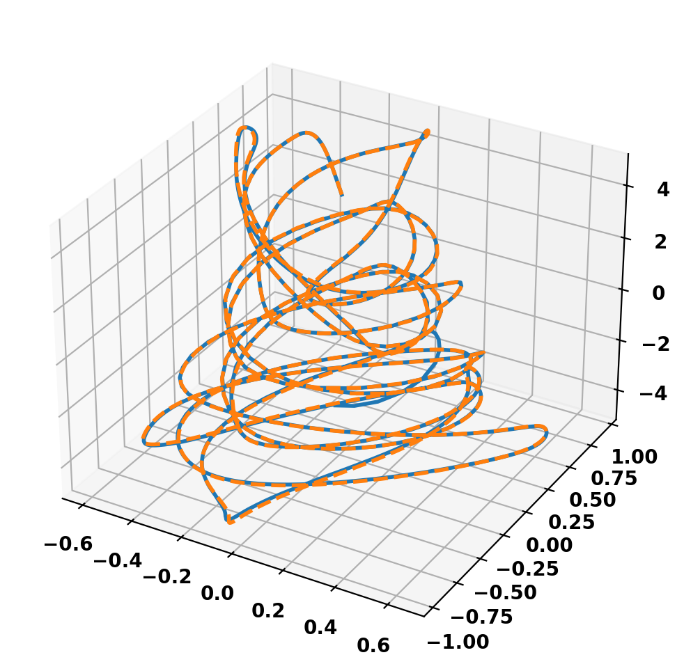
Perform field line tracing

Now we trace a single field line starting at [0.01,0.0,4.9] for both the magnetic field and the vector potential.

t = np.linspace(0, 800, 1000)
# Trace magnetic field
t0 = time.perf_counter()
sol, infodict = odeint(tracer_eval, np.array([0.01,0.0,4.9]), t, args=(binterp_obj,1.0), atol=1.E-9, full_output=True)
t1 = time.perf_counter()
print("Time = {0:.3F} [s]".format(t1-t0))
print("Time/step = {0:.2E} [s]".format((t1-t0)/np.sum(infodict['nfe'])))
print()
# Trace vector potential
t0 = time.perf_counter()
sol2, infodict = odeint(tracer_eval, np.array([0.01,0.0,4.9]), t, args=(ainterp_obj_zero_norm,3.161823), atol=1.E-9, full_output=True)
t1 = time.perf_counter()
print("Time = {0:.3F} [s]".format(t1-t0))
print("Time/step = {0:.2E} [s]".format((t1-t0)/np.sum(infodict['nfe'])))

Time = 0.661 [s]
Time/step = 1.13E-08 [s]

Time = 0.339 [s]
Time/step = 1.03E-08 [s]

Plot resulting field lines

ax = plt.figure().add_subplot(projection='3d')
ax.plot(sol[:,0],sol[:,1],sol[:,2])
ax.plot(sol2[:,0],sol2[:,1],sol2[:,2],linestyle='--')
ax.set_aspect('auto')