Inner Layer Module

The InnerLayer module solves the resistive inner-region problem of matched-asymptotic resistive-MHD stability: the thin layer around a rational surface where resistivity, inertia and the ideal singularity balance. Its output is the pair of parity-projected matching data $(\Delta_\mathrm{odd}, \Delta_\mathrm{even})$ that the outer ideal region (DCON/GPEC) matches to in order to obtain resistive growth rates, tearing $\Delta'$, and resistive interchange stability.

The module provides an abstract InnerLayerModel interface and one concrete model so far, the GGJ (Glasser–Greene–Johnson) layer, with three interchangeable solver backends. Future inner-layer models (SLAYER, kinetic layers) plug in through the same interface.

Two source papers define the equations and the asymptotic construction, and are cited by their equation numbers throughout the code and below:

GWP2016 — A. H. Glasser, Z. R. Wang and J.-K. Park, Computation of resistive instabilities by matched asymptotic expansions, Phys. Plasmas 23, 112506 (2016).
GW2020 — A. H. Glasser and Z. R. Wang, Asymptotic solutions and convergence studies of the resistive inner region equations, Phys. Plasmas 27, 012506 (2020).

Governing equations

At a rational surface the layer equations couple three fields — the perturbed flux $\Psi$ and two auxiliary layer variables $\Xi$ and $\Upsilon$ — as functions of the scaled distance $x$ from the surface. In the GWP2016 form (Eq. 11 ≡ GW2020 Eq. 1) they are

\[\begin{aligned} \Psi'' &= H\,\Upsilon' + Q\,(\Psi - x\,\Xi),\\[2pt] \Xi'' &= \frac{1}{Q^{2}}\Big[\,Q x^{2}\,\Xi - Q x\,\Psi - (E+F)\,\Upsilon - H\,\Psi'\,\Big],\\[2pt] \Upsilon''&= \frac{1}{Q}\Big[\,x^{2}\,\Upsilon - x\,\Psi - Q^{2}\big(G(\Xi-\Upsilon) - K(E\Xi + F\Upsilon + H\Psi')\big)\Big], \end{aligned}\]

where $E, F, G, H, K$ are the flux-surface-averaged equilibrium coefficients of GWP2016 Eq. (A8) and $Q$ is the dimensionless growth rate defined below. These coefficients are collected in GGJParameters.

Dimensionless scales

The layer is scaled by the local Lundquist number $S = \tau_R/\tau_A$ (ratio of resistive to Alfvén time). The displacement and growth-rate scales are

\[X_0 = S^{-1/3}, \qquad Q_0 = X_0/\tau_A \qquad \text{(GWP2016 Eqs. A14–A15)},\]

so a physical growth rate $\gamma$ maps to the scaled eigenvalue $Q = \gamma/Q_0$ (inner_Q) that appears in the equations above, and the scaled matching data are returned to physical units by the $X_0^{-2\sqrt{-D_I}} = S^{\,2\sqrt{-D_I}/3}$ rescaling (together with the $v_1^{\,2\sqrt{-D_I}}$ linear-scale factor; rescale_delta).

Mercier index and matching exponents

The premise of an inner-layer model is local Mercier stability. The Mercier interchange index and its resistive counterpart are

\[D_I = E + F + H - \tfrac14, \qquad D_R = E + F + H^2 = D_I + \big(H-\tfrac12\big)^2 \qquad \text{(GWP2016 A9–A10)},\]

(mercier_di, mercier_dr). For $D_I < 0$ the large-$x$ solutions are the two power laws $x^{r_\pm}$ with the Frobenius exponents

\[r_\pm = \tfrac32 \pm \sqrt{-D_I}, \qquad p_1 \equiv \sqrt{-D_I} \qquad \text{(GW2020 Eq. 49)}.\]

The matching datum $\Delta$ is the amplitude of the large solution $x^{r_+}$ when the small solution $x^{r_-}$ is normalized to unity (i.e. the ratio of large to small coefficient), in the physical (outer-matching) normalization. Imposing the two parities at $x=0$ (odd: $\Psi'(0)=\Xi(0)=\Upsilon(0)=0$; even: $\Psi(0)=\Xi'(0)=\Upsilon'(0)=0$) gives the pair $(\Delta_\mathrm{odd}, \Delta_\mathrm{even})$ of GWP2016 Eqs. (34)–(35).

Numerical method

Benchmark surface used in the figures

Every figure on this page is computed on the $q = 4$ rational-surface benchmark (q4_surface_benchmark) — a fixed set of GGJ layer coefficients ($S = \tau_R/\tau_A \approx 4.6\times10^{6}$, $D_I \approx -0.31$) frozen into code from the $q = 4$ rational surface of the DIII-D-like (TkMkr H-mode) equilibrium of the resistive_resmets benchmark, at that case's per-surface $\eta$ and $\rho$. The well-conditioned real-$Q$ cross-check in the Validation section instead uses the Glasser & Wang (2020) Eq. (55) surface.

Solver backends

The GGJ model exposes three solvers through the solver type parameter of GGJModel; all consume the same large-$x$ asymptotic basis and return $\Delta$ in the same convention:

backend	method	robust regime
`:shooting`	backward stable shoot from $X_\mathrm{max}\to 0$	$\lvert Q\rvert \ll 1$
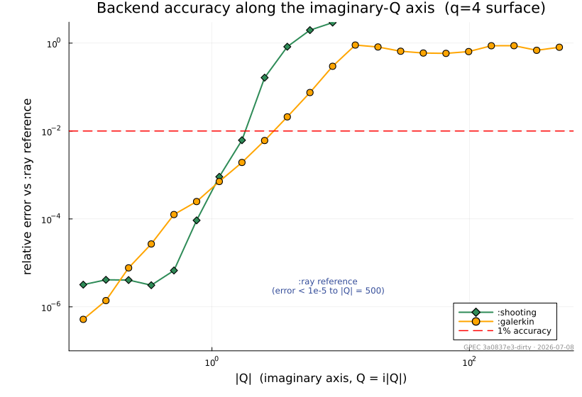
`:galerkin`	Hermite-cubic finite-element (real axis)	drift onset $\lvert Q\rvert \sim 1$; 1% error by $\lvert Q\rvert \sim 4$
`:ray` (default)	rotated-contour spectral-element collocation	$\lvert Q\rvert \sim 500$ on/near the imaginary axis

The difficulty is the large-$|Q|$ imaginary-$Q$ axis itself, where rotation and resistivity scans live: there the layer's pseudo-resonance at $x^2 = -Q^2(G+KF)$ sits directly on the real-$x$ integration path and the exponential dichotomy weakens, so both older backends degrade — :shooting through the dichotomy of the backward shoot, :galerkin through real-axis oscillation and the on-axis pseudo-resonance. (The poles of $\Delta(Q)$ itself lie on and near the real-$Q$ axis — they are the layer eigenvalues; $\Delta$ is smooth along the imaginary axis.) Measured against the :ray reference along the imaginary axis, :shooting holds to $|Q|\sim 1$ and :galerkin to $|Q|\sim 4$ (the 1% error crossings) before both lose all accuracy:

Relative error of the :shooting and :galerkin backends against the :ray reference along the imaginary-Q axis, on the q=4 benchmark surface. Each curve's crossing of the 1% line marks that method's practical reach.

The :ray backend was written to reach the large-$|Q|$ imaginary-axis regime (rotation and resistivity scans) where these fail. The remainder of this section describes it.

Entire-solution formulation

:ray works with the plain state $v = (\Psi, \Xi, \Upsilon, \Psi', \Xi', \Upsilon')$ and writes the layer equations as the first-order system

\[\frac{dv}{dx} = M(x)\,v .\]

The coefficient matrix (the GGJ internal ode_matrix) is polynomial in $x$, so $x = 0$ is an ordinary point — the $x^{-2}/x^{-4}$ singularities of the GW2020 Eq. (2) scaled form $(x\Psi,\ \Psi'/x,\ \dots)$ are artifacts of that scaling, not of the equations. Because the coefficients are entire, the system continues analytically to complex $x$, which is what makes the contour rotation below legitimate.

The rotated ray

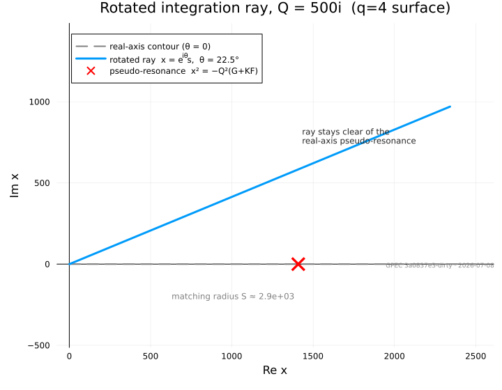
The equations are continued onto the ray

\[x = e^{i\theta}\, s, \qquad s \in [0, S], \qquad \theta = \tfrac14\arg Q,\]

The angle $\theta = \tfrac14\arg Q$ makes the parabolic-cylinder exponent of the outer solutions exactly real and clears the pseudo-resonance at $x^2 = -Q^2(G + K F)$, which on the imaginary-$Q$ axis is real and large and therefore sits directly on the un-rotated (real-$x$) contour. Rotating the contour lifts it off that point; $\theta = 0$ recovers a real-axis solve.

The rotated integration ray in the complex layer-coordinate plane at Q = 500i. The real-axis contour runs through the pseudo-resonance x² = −Q²(G+KF); the ray at θ = arg(Q)/4 = 22.5° clears it.

Spectral-element collocation BVP

On $[0, s_m]$ the system is discretized by a global Chebyshev spectral-element collocation boundary-value problem: right-biased (Radau-like) collocation at the Chebyshev–Lobatto nodes of each cell, three parity conditions at the ordinary-point origin $s = 0$, and six matching conditions at the outer edge,

\[v(S) - \Delta\, U_b - c_1 E_1 - c_2 E_2 = U_s ,\]

with the matching datum $\Delta$ and the two decaying-mode amplitudes $c_1, c_2$ carried as bordered unknowns. Here $U_s, U_b$ are the small and large power-like solutions and $E_{1,2}$ the forward-decaying exponential pair. No quantity is ever propagated across the layer, so the exponential dichotomy that limits the shooting backend never enters; the boundary condition splits it exactly.

The two parities differ only in their three $s=0$ rows, i.e. by a rank-3 update, so both are obtained from a single sparse LU factorization plus a Woodbury correction (the GGJ internal _solve_parities) rather than two factorizations. A residual-driven bisection refinement adds cells until the collocation residual meets tolerance, with a roundoff-plateau guard.

Far-field boundary and the inward march

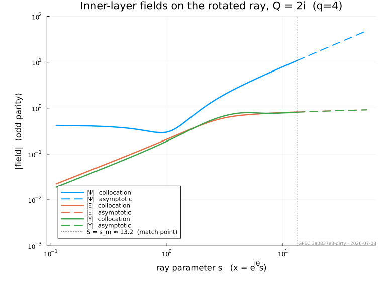
The large-$x$ boundary data use the same inps Wasow asymptotic basis as the other backends (GW2020 Eqs. 3–52), evaluated at complex $x$ by RayAsymptotics.jl and applied at the series radius $S$ where the series is trusted (residual below tolerance; pick_smax). For large $|Q|$ the trusted radius $S$ can be far outside the collocation domain $s_m$, so the power-pair data are transported inward from $S$ to $s_m$ by an L-stable 2-stage Radau IIA march in the quotient modulo the decaying exponential pair — the subspace in which $\Delta$ is defined (the GGJ internal march_boundary). An L-stable implicit method is essential: the decaying pair grows under backward integration, so any explicit marcher is stability-limited to $O(\rho S^2)$ steps, while the Radau march damps the unresolvable backward-growing directions instead of amplifying them.

The damped-zone march runs in Complex{Double64} extended precision. At large $S$ the near-parallel power-pair geometry amplifies the structured backward error of the ill-conditioned implicit solves into $\Delta$-mixing of order $10^{-4}$ at $|Q| = 500$ in Float64; extended precision removes this floor, while the well-conditioned resolved band stays in Float64.

The result is a seamless numeric↔asymptotic solution: the collocation solution on $[0, s_m]$ and the analytic $u_\mathrm{small} + \Delta\,u_\mathrm{big}$ representation for $s \ge S$ share the same power-law tail — the overlap the outer-region matching relies on.

Inner-layer fields Ψ, Ξ, Υ on the rotated ray for the q=4 surface at Q = 2i. The collocation solution (solid) joins the asymptotic representation (dashed) seamlessly at the match point S = s_m.

Validation and benchmarks

Cross-check against the Fortran rmatch solver. At the Glasser & Wang (2020) Eq. (55) operating point $Q = 0.1234$ (real) the :galerkin backend reproduces the Fortran rmatch deltac solver to $\sim 10^{-8}$:

quantity	`:galerkin` (= Fortran to $10^{-8}$)	`:ray`
$\Delta_\mathrm{odd}$	$3.698368\times 10^{4}$	$3.69789\times 10^{4}$
$\Delta_\mathrm{even}$	$14.759721$	$14.759715$

The large $\lvert\Delta_\mathrm{odd}\rvert \sim 4\times10^{4}$ means this operating point sits near a pole of $\Delta(Q)$, where every solver's error is amplified by the pole geometry; the $1.3\times10^{-4}$ :galerkin↔:ray difference in $\Delta_\mathrm{odd}$ (versus $4\times10^{-7}$ in $\Delta_\mathrm{even}$) is consistent with that amplification, not a defect of either backend.

Physical benchmark on the imaginary axis. On the $q=4$ rational-surface benchmark (q4_surface_benchmark, $S \approx 4.58\times10^6$, $D_I \approx -0.312$) the :ray backend is pinned at $Q = 500i$, a regime entirely beyond :galerkin:

quantity	value at $Q = 500i$
$\Delta_\mathrm{odd}$	$2.4720 + 13.3540\,i$
$\Delta_\mathrm{even}$	$0.13750 + 0.74275\,i$

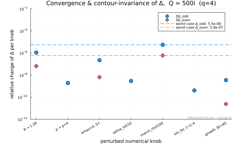
Convergence and contour invariance. Because $\Delta$ is an analytic invariant of the contour angle, re-solving with each numerical knob perturbed on an independent axis (delta_convergence) gives an honest error bar: at $Q = 500i$ the worst-case spread across all knobs is $\sim 5\times10^{-6}$ for $\Delta_\mathrm{odd}$ and $\sim 6\times10^{-7}$ for $\Delta_\mathrm{even}$. That is a single-machine error bar: across machines/BLAS builds the absolute values reproduce to $\sim 10^{-5}$ relative (the damped-zone implicit solves carry platform-dependent structured roundoff), which is why the table above quotes five significant figures.

Relative change of Δ at Q = 500i under independent perturbations of each numerical knob (contour angle, spectral order, series order/radius, refinement depth, march tolerance, handoff radius, purification depth). The worst-case spread is the reported error bar.

Choosing a backend

:ray is the default — GGJModel() constructs GGJModel{:ray}(). It is the correct choice for $|Q| \gtrsim 1$ and for any $Q$ near the imaginary axis. :galerkin remains available and may be faster for very small real $|Q|$, but note the backends take disjoint numerical-knob keywords: pass GGJModel(solver=:galerkin) explicitly when supplying the Galerkin nx/xfac knobs — passing them to the default :ray backend throws a MethodError.

using GeneralizedPerturbedEquilibrium.InnerLayer

p = q4_surface_benchmark()          # GGJParameters for the q=4 benchmark surface
γ = 500im * GGJ.q0(p)               # physical rate placing Q on the imaginary axis at 500i

Δ = solve_inner(GGJModel(), p, γ)   # (Δ_odd, Δ_even) with the default :ray backend

# Full result (raw Δ, contour, mesh, nodal solution, residuals) via solve_ray:
res = solve_ray(p, GGJ.inner_Q(p, γ))
res.Δ, res.resid, res.bc_cond

API Reference

InnerLayer

GeneralizedPerturbedEquilibrium.InnerLayer.InnerLayerModel — Type

InnerLayerModel

Abstract supertype for resistive inner-layer models. Each concrete model is a small, parameter-free type tag (often parameterized by a solver-choice symbol) that selects a solve_inner method.

Implementations live in submodules of InnerLayer, e.g. InnerLayer.GGJ.

field	meaning
`E`	Glasser interchange parameter (enters Mercier `D_I = E+F+H−¼`)
`F`	Glasser interchange parameter
`G`	Coupling coefficient (curvature × pressure gradient)
`H`	Pfirsch–Schlüter coefficient
`K`	Glasser parameter
`M`	Mercier-related auxiliary parameter (held but not used here)
`taua`	Local Alfvén time at the rational surface
`taur`	Local resistive time at the rational surface
`v1`	Linear scale factor used in the V₁ rescaling
`ising`	Index of the singular surface (traceability only)