Ballooning and Mercier Local Stability

This note describes the physical and mathematical foundations of Bal.jl, which computes local Mercier and high-$n$ ballooning stability. It covers the ballooning-mode equation, the asymptotic boundary treatment, and the local perturbation framework used to generate the $s$-$\alpha$ diagram.

Ballooning-mode equation

Ballooning representation

In a tokamak equilibrium, physical quantities are periodic in the poloidal angle $\theta$ and toroidal angle $\zeta$. The perturbation function $\varphi$ satisfies

\[\varphi(\psi, \theta, \beta) = \varphi(\psi, \theta, \beta + 1) = \varphi(\psi, \theta + 1, \beta - q),\]

where $q$ is the safety factor.

Ballooning modes have long wavelengths along magnetic field lines and short wavelengths perpendicular to the field. They are represented using a covering-space function $\hat{\varphi}$, defined on $-\infty < \theta < \infty$:

\[\varphi(\psi, \theta, \beta) = \sum_{l=-\infty}^{\infty} \hat{\varphi}(\psi, \theta - l) \exp[-2\pi i n(\beta + lq)].\]

Here

\[\beta = \zeta - q\theta + \int q'\theta_0(\psi)\,d\psi\]

is the Clebsch coordinate. The wave-number vector contains a secular term from the magnetic shear $q'$:

\[|\nabla\beta|^2 = |\nabla\zeta - q\nabla\theta|^2 + q'^2(\theta-\theta_0)^2|\nabla\psi|^2 - 2q'(\theta-\theta_0)(\nabla\zeta-q\nabla\theta)\cdot\nabla\psi.\]

Ideal marginal ballooning equation

At the stability boundary, $\gamma = 0$. Variation of the ideal-MHD energy principle gives the ballooning ODE

\[\mathbf{B}\cdot\nabla \left( \frac{|\nabla\beta|^2}{B^2} \mathbf{B}\cdot\nabla\hat{\varphi} \right) + 2\frac{P'}{\chi'}\kappa_w\hat{\varphi} = 0,\]

where $\chi$ is the poloidal flux and $P'$ is the pressure-gradient term used by the local-stability equations. Written using the Jacobian $\mathcal{J}$,

\[\frac{\chi'}{\mathcal{J}}\frac{\partial}{\partial\theta} \left( \frac{|\nabla\beta|^2}{B^2} \frac{\chi'}{\mathcal{J}} \frac{\partial\hat{\varphi}}{\partial\theta} \right) + 2\frac{P'}{\chi'}\kappa_w\hat{\varphi} = 0.\]

Bal.jl converts this to a first-order matrix equation,

\[\frac{\partial\mathbf{u}}{\partial\theta} = \mathbf{L}\mathbf{u}, \qquad \mathbf{u} = \begin{pmatrix} \hat{\varphi} \\ \dfrac{|\nabla\beta|^2}{B^2} \dfrac{\chi'}{\mathcal{J}} \dfrac{\partial\hat{\varphi}}{\partial\theta} \end{pmatrix},\]

with

\[\mathbf{L} = \frac{\mathcal{J}}{\chi'} \begin{pmatrix} 0 & \dfrac{B^2}{|\nabla\beta|^2} \\ -2\dfrac{P'}{\chi'}\kappa_w & 0 \end{pmatrix}.\]

Curvature decomposition

The instability drive is the projected curvature

\[\kappa_w \equiv \frac{\boldsymbol{\kappa}\times\mathbf{B}}{B^2}\cdot\nabla\beta.\]

Using $\nabla\beta = \nabla\zeta - q\nabla\theta - q'\theta\nabla\psi$, the curvature separates into non-secular and secular pieces:

\[\kappa_w = \kappa_n - q'\theta\kappa_s,\]

where

\[\kappa_s \equiv \frac{\boldsymbol{\kappa}\times\mathbf{B}}{B^2}\cdot\nabla\psi = -\frac{\pi f}{\mathcal{J}} \frac{\partial}{\partial\theta} \left(\frac{1}{B^2}\right).\]

This decomposition is the main structure used to assemble the ballooning coefficient matrix.

Asymptotic basis and Mercier exponent

In the $\theta\to\infty$ limit, the coefficient matrix diverges because $|\nabla\beta|^2 \simeq q'^2\theta^2|\nabla\psi|^2$. Bal.jl applies the canonical transformation

\[\mathbf{R} = \operatorname{diag}(\theta^{-1/2}, \theta^{1/2})\]

and solves

\[\frac{\partial\mathbf{v}}{\partial\theta} = \mathbf{M}\mathbf{v}, \qquad \mathbf{M} = \begin{pmatrix} \dfrac{1}{2\theta} & \dfrac{\mathcal{J}}{\chi'} \dfrac{B^2\theta}{|\nabla\beta|^2} \\ -\dfrac{\mathcal{J}}{\chi'} \dfrac{2P'\kappa_w}{\chi'\theta} & -\dfrac{1}{2\theta} \end{pmatrix}.\]

To keep the lowest-order matrix finite, the code applies

\[\mathbf{S} = \begin{pmatrix} 1 & 0 \\ \sigma & 1 \end{pmatrix}, \qquad \sigma = -\frac{2\pi f P'q'}{\chi'^2 B^2}.\]

The transformed matrices $\mathbf{N}_k = \mathbf{S}^{-1}\mathbf{M}_k\mathbf{S}$ enter the recurrence relation

\[\frac{\partial\mathbf{w}^{(k+1)}}{\partial\theta} = [\mathbf{N}_0-(\alpha+k)\mathbf{I}]\mathbf{w}^{(k)} + \sum_{l=1}^{k}\mathbf{N}_l\mathbf{w}^{(k-l)}.\]

The Mercier exponent $\alpha$ follows from the zeroth-order solvability condition:

\[\det[\langle\mathbf{N}_0\rangle-\alpha\mathbf{I}] = 0, \qquad \alpha = \pm\sqrt{-D_I}.\]

Equivalence with the surface-average Mercier formula

The previous Mercier.jl evaluated the Mercier index from flux-surface averages. The two routes are mathematically equivalent: they are different reductions of the same large-$\theta$ ballooning solvability condition.

Let the flux-surface average used by the old implementation be

\[\langle X\rangle_{\mathrm{fs}} \equiv \int_0^1 \frac{\mathcal{J}}{V'} X(\theta)\,d\theta,\]

and define

\[A_1 = \left\langle\frac{B^2}{|\nabla\psi|^2}\right\rangle_{\mathrm{fs}}, \qquad A_2 = \left\langle\frac{1}{|\nabla\psi|^2}\right\rangle_{\mathrm{fs}},\]

\[A_3 = \left\langle\frac{1}{B^2}\right\rangle_{\mathrm{fs}}, \qquad A_4 = \left\langle\frac{1}{B^2|\nabla\psi|^2}\right\rangle_{\mathrm{fs}}, \qquad A_5 = \left\langle B^2\right\rangle_{\mathrm{fs}}.\]

Below, an overbar denotes the period integral used to form the Bal.jl $\bar{d}_0$ matrix:

\[\overline{X} \equiv \int_0^1 X(\theta)\,d\theta.\]

With $F = 2\pi f$, the old code evaluated

\[T = \frac{F P' V'}{q'\chi'^3} A_2,\]

and then

\[D_I^{\mathrm{avg}} = -\frac14 + T(1-T) + P'\left(\frac{V'}{q'\chi'^2}\right)^2 A_1 \left[ P'\left(A_3+\frac{F^2}{\chi'^2}A_4\right) - \frac{V''}{V'} \right].\]

This is the surface-average Mercier expression that appeared in the old Mercier.jl and, temporarily, in the earlier resistive_interchange helper. The associated GGJ resistive-interchange quantity used

\[H = \frac{F P' V'}{q'\chi'^3} \left( A_2 - \frac{A_1}{A_5} \right), \qquad D_R = D_I + \left(H-\frac12\right)^2.\]

The determinant route starts from the same ballooning equation, takes the large-$\theta$ limit, applies the $\mathbf{R}$ and $\mathbf{S}$ transformations, and obtains the periodic lowest-order system

\[\frac{\partial\mathbf{w}^{(1)}}{\partial\theta} = (\mathbf{N}_0-\alpha\mathbf{I})\mathbf{w}^{(0)}.\]

Solvability requires the mean operator to have a null vector:

\[[\overline{\mathbf{N}_0}-\alpha\mathbf{I}]\mathbf{w}^{(0)}=0.\]

The transformed matrix is traceless by construction,

\[\operatorname{tr}\overline{\mathbf{N}_0} = 0,\]

so the characteristic equation reduces to

\[\alpha^2 + \det\overline{\mathbf{N}_0} = 0.\]

Comparing this with the Mercier exponent definition $\alpha^2 = -D_I$ gives

\[D_I = \det\overline{\mathbf{N}_0}.\]

The reduction can be written explicitly. For the unperturbed Mercier scan, $\mathbf{N}_0$ has the code form

\[\mathbf{N}_0(\theta) = \begin{pmatrix} \frac12 + M_{12}\sigma & M_{12} \\ M_{21}-\sigma-M_{12}\sigma^2 & -\frac12-M_{12}\sigma \end{pmatrix},\]

where

\[M_{12} = \frac{\mathcal{J}}{\chi'} \frac{B^2}{q'^2|\nabla\psi|^2}, \qquad M_{21} = -2\frac{\mathcal{J}}{\chi'^2}P'\kappa_n, \qquad \sigma = -\frac{F P' q'}{\chi'^2 B^2}.\]

The averaged matrix can therefore be written as

\[\bar{d}_0 \equiv \overline{\mathbf{N}_0} = \begin{pmatrix} \frac12+B & A \\ K & -\frac12-B \end{pmatrix},\]

with

\[A = \overline{M_{12}}, \qquad B = \overline{M_{12}\sigma}, \qquad K = \overline{M_{21}-\sigma-M_{12}\sigma^2}.\]

The first two averages are direct:

\[A = \frac{V'}{q'^2\chi'}A_1,\]

\[B = \overline{ \frac{\mathcal{J}}{\chi'} \frac{B^2}{q'^2|\nabla\psi|^2} \left( -\frac{F P' q'}{\chi'^2B^2} \right) } = -\frac{F P' V'}{q'\chi'^3}A_2 = -T.\]

For $K$, separate the three pieces:

\[K = \overline{M_{21}} -\overline{\sigma} -\overline{M_{12}\sigma^2}.\]

The last term is also direct:

\[\overline{M_{12}\sigma^2} = \overline{ \frac{\mathcal{J}}{\chi'} \frac{B^2}{q'^2|\nabla\psi|^2} \frac{F^2P'^2q'^2}{\chi'^4B^4} } = \frac{F^2P'^2V'}{\chi'^5}A_4.\]

The remaining curvature combination reduces by the axisymmetric equilibrium identity used in the Mercier derivation:

\[\int_0^1 \left( 2\mathcal{J}\kappa_n - \frac{Fq'}{B^2} \right)d\theta = \frac{V'}{\chi'} \left( P'A_3 - \frac{V''}{V'} \right).\]

Using $M_{21}=-2\mathcal{J}P'\kappa_n/\chi'^2$ and $\sigma=-FP'q'/(\chi'^2B^2)$, this gives

\[\overline{M_{21}}-\overline{\sigma} = -\frac{P'}{\chi'^2} \int_0^1 \left( 2\mathcal{J}\kappa_n - \frac{Fq'}{B^2} \right)d\theta = -\frac{P'V'}{\chi'^3} \left( P'A_3 - \frac{V''}{V'} \right).\]

Therefore

\[K = -\frac{P'V'}{\chi'^3} \left[ P'\left(A_3+\frac{F^2}{\chi'^2}A_4\right) - \frac{V''}{V'} \right].\]

Now take the determinant:

\[\det\bar{d}_0 = \left(\frac12+B\right)\left(-\frac12-B\right)-AK.\]

Substituting $B=-T$ gives the first part of the old Mercier expression:

\[\left(\frac12-T\right)\left(-\frac12+T\right) = -\frac14+T(1-T).\]

Substituting $A$ and $K$ gives the second part:

\[-AK = \frac{V'}{q'^2\chi'}A_1 \frac{P'V'}{\chi'^3} \left[ P'\left(A_3+\frac{F^2}{\chi'^2}A_4\right) - \frac{V''}{V'} \right]\]

\[= P'\left(\frac{V'}{q'\chi'^2}\right)^2 A_1 \left[ P'\left(A_3+\frac{F^2}{\chi'^2}A_4\right) - \frac{V''}{V'} \right].\]

Thus the determinant route gives exactly

\[\det\bar{d}_0 = -\frac14 + T(1-T) + P'\left(\frac{V'}{q'\chi'^2}\right)^2 A_1 \left[ P'\left(A_3+\frac{F^2}{\chi'^2}A_4\right) - \frac{V''}{V'} \right] = D_I^{\mathrm{avg}}.\]

So, under the same normalization and exact equilibrium identities,

\[D_I^{\mathrm{det}} \equiv \det(\bar{d}_0) = D_I^{\mathrm{avg}}.\]

The implementation difference is numerical rather than physical. The old surface-average route evaluates the closed Mercier formula directly, while the new Bal.jl route constructs the same Mercier index from the averaged large-$\theta$ local-mode matrix. In finite-precision calculations the two can separate near the magnetic axis or other ill-conditioned surfaces because both forms contain factors such as $1/q'$ and $1/q'^2$. Away from those regions, they should agree to the accuracy of the equilibrium derivatives and surface quadrature.

The divergent big solution and decaying small solution have leading forms

\[\mathbf{u}_{\mathrm{large}}^{(0)} \simeq \begin{pmatrix} \theta^{\alpha-1/2} \\ \theta^{\alpha+1/2}(\sigma+w_{21}) \end{pmatrix}, \qquad \mathbf{u}_{\mathrm{small}}^{(0)} \simeq \begin{pmatrix} \theta^{-\alpha-1/2} \\ \theta^{-\alpha+1/2}(\sigma+w_{22}) \end{pmatrix}.\]

First-order asymptotic matching

The zeroth-order large-$\theta$ solution alone is not accurate enough at a finite integration boundary $\theta_{\max}$. Bal.jl therefore includes the first-order correction $\mathbf{w}^{(1)}$:

\[\frac{\partial\mathbf{w}^{(1)}}{\partial\theta} = (\mathbf{N}_0-\alpha\mathbf{I})\mathbf{w}^{(0)} = \tilde{\mathbf{N}}_0(\theta)\mathbf{w}^{(0)}.\]

The first-order solution is written as

\[\mathbf{w}^{(1)}(\theta) = \left(\int\tilde{\mathbf{N}}_0(\theta)\,d\theta\right)\mathbf{w}^{(0)} + \mathbf{c}^{(1)} \equiv \tilde{\mathbf{w}}^{(1)}(\theta) + \mathbf{c}^{(1)}.\]

The constant vector is fixed by the first-order solvability condition,

\[[\langle\mathbf{N}_0\rangle-(\alpha+1)\mathbf{I}]\mathbf{c}^{(1)} = - \left\langle [\mathbf{N}_0-(\alpha+1)\mathbf{I}] \tilde{\mathbf{w}}^{(1)}(\theta) + \mathbf{N}_1\mathbf{w}^{(0)} \right\rangle.\]

This gives the asymptotic boundary form

\[\mathbf{u}_{\mathrm{boundary}} \simeq \mathbf{R}\mathbf{S} \left( \mathbf{w}^{(0)} + \frac{1}{\theta}\mathbf{w}^{(1)}(\theta) \right).\]

Local thin-layer ordering

The $s$-$\alpha$ diagram scans local instability near a flux surface $\psi_b$ without recomputing the full equilibrium. A thin-layer parameter $0 < \mu \ll 1$ is introduced through

\[s = \frac{\psi-\psi_b}{\mu}, \qquad \frac{\partial}{\partial\psi} = \frac{1}{\mu}\frac{\partial}{\partial s}.\]

Profiles are expanded as background plus local perturbation,

\[P(\psi) = P^{(0)}(\psi) + \mu P^{(1)}(s) + \cdots, \qquad q(\psi) = q^{(0)}(\psi) + \mu q^{(1)}(s) + \cdots.\]

After differentiation, the $\mu$ amplitude cancels the $1/\mu$ derivative scale. Thus the derivative-level perturbations are order unity:

\[P_\psi = P_\psi^{(0)} + P_s^{(1)}, \qquad q_\psi = q_\psi^{(0)} + q_s^{(1)}.\]

The subscript $s$ therefore represents the promoted local derivative perturbation used as the practical scan variable in the $s$-$\alpha$ diagram. Retained first-order contributions are denoted by a superscript $[1]$; for example, $I_{\mathrm{per}}^{[1]}$ is the retained local periodic variation of the integrated shear.

Local $P'$ and $q'$ perturbations

Using the integrated-shear function

\[I_{\mathrm{tot}} = q'(\theta-\theta_k) + I_{\mathrm{per}},\]

the wave-number space and curvature are written

\[\left(\frac{|\nabla\beta|}{B}\right)^2 = \frac{1}{\chi'^2|\nabla\psi|^2} + \frac{|\nabla\psi|^2}{B^2}I_{\mathrm{tot}}^2,\]

\[\kappa_w = \frac{\boldsymbol{\kappa}\cdot\nabla\psi} {\chi'|\nabla\psi|^2} - \kappa_s I_{\mathrm{tot}}.\]

With

\[I_{\mathrm{tot}} = I_{\mathrm{tot}}^{(0)} + I_{\mathrm{tot}}^{[1]}, \qquad I_{\mathrm{tot}}^{[1]} = q_s^{(1)}(\theta-\theta_k) + I_{\mathrm{per}}^{[1]},\]

the retained order-unity perturbation terms are

\[\left(\frac{|\nabla\beta|^2}{B^2}\right)_{O(1),\mathrm{ret}} = \frac{|\nabla\psi|_0^2}{B_0^2} \left[ 2I_{\mathrm{tot}}^{(0)}I_{\mathrm{tot}}^{[1]} + \left(I_{\mathrm{tot}}^{[1]}\right)^2 \right],\]

\[\kappa_w^{[1]} = -\kappa_s^{(0)}I_{\mathrm{tot}}^{[1]}.\]

The cross term and nonlinear $(I_{\mathrm{tot}}^{[1]})^2$ term are retained in the matrix assembly rather than discarded by linearization.

$\mathbf{N}_0$ matrix construction

The lower-triangular element of the canonical transformation combines the local $P'$ and $q'$ perturbations:

\[\sigma = -\frac{2\pi f}{\chi_0'^2B_0^2} \left(P_\psi^{(0)} + P_s^{(1)}\right) \left(q_\psi^{(0)} + q_s^{(1)}\right).\]

The $(1,2)$ component of the asymptotic matrix responds to $q_s^{(1)}$:

\[(\mathbf{M}_0)_{12} = \frac{\mathcal{J}_0}{\chi_0'} \frac{B_0^2} {\left(q_\psi^{(0)}+q_s^{(1)}\right)^2|\nabla\psi|_0^2}.\]

The $(2,1)$ component uses the expanded non-secular curvature,

\[\kappa_n(\theta) = \kappa_n^{(0)}(\theta) + \kappa_s^{(0)}(\theta)q_s^{(1)}\theta_k - \kappa_s^{(0)}(\theta)I_{\mathrm{per}}^{[1]}(\theta),\]

which gives

\[(\mathbf{M}_0)_{21} = -\frac{2\mathcal{J}_0}{\chi_0'^2} \left(P_\psi^{(0)} + P_s^{(1)}\right) \left[ \kappa_n^{(0)}(\theta) + \kappa_s^{(0)}(\theta)q_s^{(1)}\theta_k - \kappa_s^{(0)}(\theta)I_{\mathrm{per}}^{[1]}(\theta) \right].\]

The final matrix $\mathbf{N}_0(\theta)=\mathbf{S}^{-1}\mathbf{M}_0(\theta)\mathbf{S}$ is period-averaged to form $\langle\mathbf{N}_0\rangle$ in the Mercier solvability equation.

$\mathbf{N}_1$ correction

The first-order asymptotic boundary condition requires the $O(\theta^{-2})$ matrix $\mathbf{N}_1$. In the large-$\theta$ limit, only the upper-right component of $\mathbf{M}_1$ remains:

\[\mathbf{M}_1(\theta) = \begin{pmatrix} 0 & a_1(\theta) \\ 0 & 0 \end{pmatrix},\]

where

\[a_1(\theta) = -2\frac{\mathcal{J}_0}{\chi_0'} \frac{B_0^2} {|\nabla\psi|_0^2\left(q_\psi^{(0)}+q_s^{(1)}\right)^3} \left[ I_{\mathrm{per}}^{(0)}(\theta) + I_{\mathrm{per}}^{[1]}(\theta) - \left(q_\psi^{(0)}+q_s^{(1)}\right)\theta_k \right].\]

Applying the $\mathbf{S}^{-1}$ transformation gives

\[\mathbf{N}_1(\theta) = a_1(\theta) \begin{pmatrix} \sigma & 1 \\ -\sigma^2 & -\sigma \end{pmatrix}.\]

Thus $\mathbf{N}_1$ is closed in terms of $I_{\mathrm{per}}^{[1]}$, $P_s^{(1)}$, and $q_s^{(1)}$. The $I_{\mathrm{per}}^{[1]}$ and $q_s^{(1)}$ terms control $a_1(\theta)$, while $P_s^{(1)}$ enters through $\sigma$.

Practical implementation in Bal.jl

Geometric curvature formula

The non-secular curvature calculation uses the geometric expression

\[\kappa_n^{(0)} = -\frac{1}{\mathcal{J}_0B_0} \frac{\partial}{\partial\psi} \left(\frac{\mathcal{J}_0B_0}{\chi'_0}\right) + \frac{1}{\mathcal{J}_0B_0} \frac{\partial}{\partial\theta} \left( \mathcal{J}_0 \frac{\mathbf{B}_0\cdot\nabla\theta\times\nabla\zeta}{B_0} \right) + \frac{2\pi f q'_0}{B_0^2\mathcal{J}_0}.\]

This avoids relying entirely on Grad-Shafranov identities, which can amplify numerical equilibrium errors near the edge or in other regions where the input equilibrium does not satisfy the Grad-Shafranov equation exactly.

Two-loop structure

The code separates the calculation into two loops to avoid repeatedly differentiating noisy geometric quantities.

• Loop 1: Use only unperturbed background quantities, such as $P'$ and $q'$, to precompute the base structural curvature $\kappa_n^{(0)}$.
• Loop 2: Insert the requested local perturbations, such as $P_s^{(1)}$, $q_s^{(1)}$, and $I_{\mathrm{per}}^{[1]}$. The code adds only the analytically derived algebraic perturbation ``\kappas^{(0)}qs^{(1)}\theta_k
  • \kappas^{(0)}I{\mathrm{per}}^{[1]}`` to the precomputed
  $\kappa_n^{(0)}$.

This preserves the perturbation structure while avoiding unstable repeated geometric differentiation.

$\theta_{\max}$ and Baloo.f-style matching

For large $\theta$, the wave-number factor behaves like a quadratic polynomial,

\[a_2\theta^2 + a_1\theta + a_0 = a_2\left(\theta+\frac{a_1}{2a_2}\right)^2 + \left(a_0-\frac{a_1^2}{4a_2}\right).\]

The residual scale is $c = a_0-a_1^2/(4a_2)$. To make the asymptotic approximation valid, the code chooses an integration boundary where the $\theta^2$ term dominates, using the scale $\sqrt{|c/a_2|}$. Because the shooting boundary is a single flux-surface quantity, Bal.jl evaluates this scale on the ballooning theta grid and uses the largest finite value on that surface. The base integration boundary is then capped as $\theta_{\max}=\min(16.5,10\max_\theta\sqrt{|c/a_2|})$.

Directly extracting $c_{a1}$ or $\Delta'$ from the small asymptotic solution is numerically fragile. The comparison below shows that the Baloo.f style, which sets the displacement to vanish at $\pm\theta_{\max}$ and computes $\Delta'$ from the resulting solution, gives the most stable continuous profile.

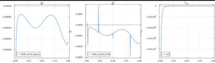
Bal.jl therefore adopts the Baloo.f-style boundary replacement for the ballooning $\Delta'$ calculation.

Ballooning angle and integral-gauge correction

The ballooning angle $\theta_k$ is the integration constant specifying where the total accumulated local shear is zero:

\[I_{\mathrm{tot}}(\theta_k) = 0.\]

In Bal.jl,

\[I_{\mathrm{tot}} = \left(q'^{(0)}+q_s^{(1)}\right)(\theta-\theta_k) + \left(I_{\mathrm{per}}^{(0)}(\theta) + I_{\mathrm{per}}^{[1]}(\theta)\right).\]

To satisfy the gauge exactly, the periodic shear functions are shifted so that they vanish at $\theta_k$:

\[I_{\mathrm{per}}^{(0)}(\theta) \leftarrow I_{\mathrm{per}}^{(0)}(\theta) - I_{\mathrm{per}}^{(0)}(\theta_k),\]

\[I_{\mathrm{per}}^{[1]}(\theta) \leftarrow I_{\mathrm{per}}^{[1]}(\theta) - I_{\mathrm{per}}^{[1]}(\theta_k).\]

This aligns the numerical implementation with the theoretical gauge used in the ballooning formulation.

locstab_fs outputs

Bal.jl now computes both the Mercier criterion and the ballooning $\Delta'$. The previous standalone Mercier.jl path can therefore be removed from the local stability calculation. The comparison below shows agreement between the previous Mercier calculation and the new Bal.jl calculation.

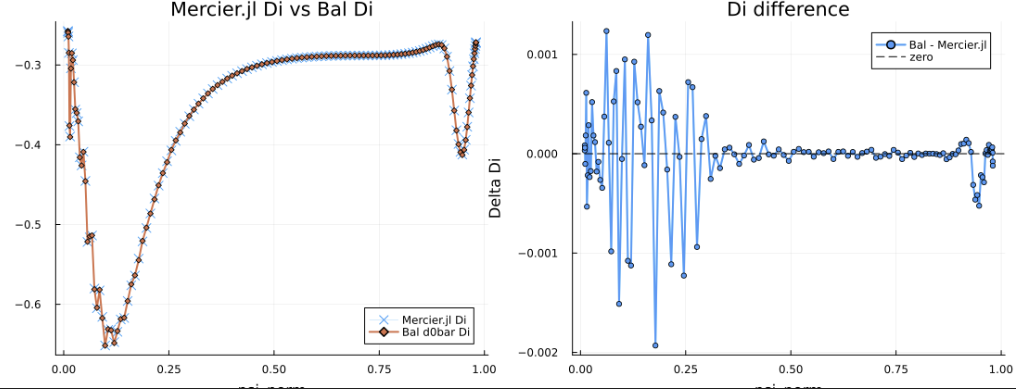
The local-stability output now stores ballooning $\Delta'$ in the fourth locstab_fs entry. In the HDF5 output this is written as locstab/ballooning_Delta_prime, distinct from the tearing $\Delta'$ outputs under singular/ and perturbed_equilibrium/singular_coupling/.